INTERVIEW PREP TOPICS OVERVIEW

• writing code on a whiteboard (see Recommendations Combined.docx)
• details of O(nlogn) sorts (at least one, maybe quick sort and merge sort - merge sort can be highly useful in situations where quick sort is impractical: which ones?);
• binary search (write and debug); other search algos?
• Optional, from another article: know at least one flavor of balanced binary tree: red/black, splay or AVL tree (how it's implemented)
• hashtables: the single most important data structure; know how they work; implement one using only arrays during the interview (45 min);
• edit distance and other DP algos;
• BST traversals (various, left-to-right, etc.);
• BFS & DFS, and know the difference between inorder, postorder and preorder. More here;
• Graphs - important at Google; 3 representations in memory (objects and pointers, matrix, and adjacency list); know each representation, pros & cons. Implement basic graph traversal algorithms: BFS & DFS (computational complexity, tradeoffs).

Optional, from another article: * Study fancier graph algorithms: Dijkstra and A* - they're really great. ADVICE: if you get any problem - first think graphs: fundamental and flexible way of representing relationships, 50-50 chance that any interesting design problem has a graph involved! * Learn data structures and algos, should especially know the most famous classes of NP-complete problems (traveling salesman and knapsack) => recognize them when in disguise; and what NP-complete means * Descrete Math (counting problems, probability problems, and other Discrete Math 101 situations) * OS: threads and concurrency; locks, mutexes, semaphores, monitors - how they work; deadlock, livelock - how to avoid. What resources a process needs, a thread needs, how context switching works, how it's initiated by OS and underlying hardware. Know a little about scheduling.

Data Structures and Algorithms: * Karya Umum Dsa; * Geeks for Geeks: 500 Data Structures and Algorithms; * Top 10 Algos in Interview Questions; * Big-O Cheat Sheet and Big-O notation. * Competitive Programmer's Handbook

Websites Recommended by Google Software Engineers for practice: * Top Coder: https://www.topcoder.com/ * HackerRank: https://www.hackerrank.com/ * Project Euler: https://projecteuler.net/ * LeetCode: LeetCode.com * Interview Cake: https://www.interviewcake.com/ * CodeFights https://codefights.com/

Second company:
Critical
* Arrays and lists * Stacks and queues * Binary trees, Graphs, Graph traversals: BFS, DFS * Search: iterator, binary, hash * Sort: merge, quick, bucket * Hash tables * Recursion * Complexity, Big O notation

Nice to Have * Trie * Red-black trees (theory) * Randomized quicksort (theory) * Spanning tree, minimum cut (theory) * Heap - part of heap sort (heapify) * Radix sort (theory) * Dynamic programming (However: there is no need to learn or know how to do dynamic programming or memorization) * Set

Another website for pratice: https://leetcode.com/problemset/all/

SORTING ALGORITHMS (nLogn)

Quick Sort (other verions)

Comment for the second solution

• First call - consider all the elements (arr[0 : n-1].
• If pivot's index = k, repeat the process for elements [0 : k-1] and [k+1 : n-1].
• While sorting the elements from k+1 to n-1, the current pivot would end up in some position p. We'd then sort the elements from k+1 to p-1 and p+1 to n-1, and so on.
• Pivot as first or last element => bad performance on sorted lists, but still most operationally efficient (has to be done repeatedly; choosing a random pivot - expensive). One can also pick an element from the middle

# second in-place algo
def quick_sort2(array, start, end):
        
    if start >= end:
        return

    p = partition2(array, start, end)
    quick_sort2(array, start, p-1)
    quick_sort2(array, p+1, end)
    
    
def partition2(array, start, end):
        
    pivot = array[start]
    low = start + 1
    high = end

    while True:
        # if current value > pivot => OK, move left,keep track of low pointer (to know when all moved)
        while low <= high and array[high] >= pivot:
            high = high - 1

        # Opposite to the above
        while low <= high and array[low] <= pivot:
            low = low + 1

        # either found an out-of-order value for high and low OR low > high => exit loop
        if low <= high:
            array[low], array[high] = array[high], array[low]    # loop continues            
        else:            
            break                                                # exit loop

    array[start], array[high] = array[high], array[start]

    return high

# is this really a 3-way quick sort? + how can I get rid of random?
# https://stackoverflow.com/questions/36972714/implementing-3-way-quicksort
import random
def quick_sort_3way(a, l, r):
    if l >= r:
        return
    k = random.randint(l, r)
    a[l], a[k] = a[k], a[l]
    m1, m2 = partition3(a, l, r)
    quick_sort_3way(a, l, m1 - 1)
    quick_sort_3way(a, m2 + 1, r)

def partition3(a, l, r):
    x, j, t = a[l], l, r
    i = j

    while i <= t :
        if a[i] < x:
            a[j], a[i] = a[i], a[j]
            j += 1

        elif a[i] > x:
            a[t], a[i] = a[i], a[t]
            t -= 1
            i -= 1 # remain in the same i in this case
        i += 1   
    return j, t

# short version of quicksort - not in place, requires storage
def quick_sort3(_list):
    
    if len(_list) <= 1:
        return _list
    
    pivot = _list[len(_list) // 2]                       # it can also be first or last element of the list
    left = [x for x in _list if x < pivot]
    middle = [x for x in _list if x == pivot]
    right = [x for x in _list if x > pivot]
        
    return quick_sort3(left) + middle + quick_sort3(right)

# test sorting f(x)
a, b, c, d = [8, 7, 4, 2, 1, 25, 29, 38, 45, 5, 101, 97, 73, 74, 72, 55], [8, 7, 4, 2, 1], [8, 7, 2, 11], [8, 7]
for arr in [a, b, c, d]:
    print(arr, end=' ')
    quick_sort(arr, 0, len(arr) - 1)      # in-place sorting    
    print('=> ', arr)
    #print('=> ', quick_sort3(arr))       # not in-place

Partition: pivot =  55
partition: i =  -1
Before last swap: [8, 7, 4, 2, 1, 25, 29, 38, 45, 5, 101, 97, 73, 74, 72, 55]
After last swap: [8, 7, 4, 2, 1, 25, 29, 38, 45, 5, 55, 97, 73, 74, 72, 101]

Partition: pivot =  5
partition: i =  -1
Before last swap: [4, 2, 1, 7, 8, 25, 29, 38, 45, 5, 55, 97, 73, 74, 72, 101]
After last swap: [4, 2, 1, 5, 8, 25, 29, 38, 45, 7, 55, 97, 73, 74, 72, 101]

Partition: pivot =  1
partition: i =  -1
Before last swap: [4, 2, 1, 5, 8, 25, 29, 38, 45, 7, 55, 97, 73, 74, 72, 101]
After last swap: [1, 2, 4, 5, 8, 25, 29, 38, 45, 7, 55, 97, 73, 74, 72, 101]

Partition: pivot =  4
partition: i =  0
Before last swap: [1, 2, 4, 5, 8, 25, 29, 38, 45, 7, 55, 97, 73, 74, 72, 101]
After last swap: [1, 2, 4, 5, 8, 25, 29, 38, 45, 7, 55, 97, 73, 74, 72, 101]

Recursive call for [1, 2]
Recursive call for [5, 8, 25, 29, 38, 45, 7, 55, 97, 73, 74, 72, 101]
Recursive call for []
Recursive call for [2, 4, 5, 8, 25, 29, 38, 45, 7, 55, 97, 73, 74, 72, 101]
Partition: pivot =  7
partition: i =  3
Before last swap: [1, 2, 4, 5, 8, 25, 29, 38, 45, 7, 55, 97, 73, 74, 72, 101]
After last swap: [1, 2, 4, 5, 7, 25, 29, 38, 45, 8, 55, 97, 73, 74, 72, 101]

Partition: pivot =  8
partition: i =  4
Before last swap: [1, 2, 4, 5, 7, 25, 29, 38, 45, 8, 55, 97, 73, 74, 72, 101]
After last swap: [1, 2, 4, 5, 7, 8, 29, 38, 45, 25, 55, 97, 73, 74, 72, 101]

Partition: pivot =  25
partition: i =  5
Before last swap: [1, 2, 4, 5, 7, 8, 29, 38, 45, 25, 55, 97, 73, 74, 72, 101]
After last swap: [1, 2, 4, 5, 7, 8, 25, 38, 45, 29, 55, 97, 73, 74, 72, 101]

Partition: pivot =  29
partition: i =  6
Before last swap: [1, 2, 4, 5, 7, 8, 25, 38, 45, 29, 55, 97, 73, 74, 72, 101]
After last swap: [1, 2, 4, 5, 7, 8, 25, 29, 45, 38, 55, 97, 73, 74, 72, 101]

Partition: pivot =  38
partition: i =  7
Before last swap: [1, 2, 4, 5, 7, 8, 25, 29, 45, 38, 55, 97, 73, 74, 72, 101]
After last swap: [1, 2, 4, 5, 7, 8, 25, 29, 38, 45, 55, 97, 73, 74, 72, 101]

Recursive call for [1, 2, 4, 5, 7, 8, 25, 29]
Recursive call for [45, 55, 97, 73, 74, 72, 101]
Recursive call for [1, 2, 4, 5, 7, 8, 25]
Recursive call for [38, 45, 55, 97, 73, 74, 72, 101]
Recursive call for [1, 2, 4, 5, 7, 8]
Recursive call for [29, 38, 45, 55, 97, 73, 74, 72, 101]
Recursive call for [1, 2, 4, 5, 7]
Recursive call for [25, 29, 38, 45, 55, 97, 73, 74, 72, 101]
Recursive call for [1, 2, 4, 5]
Recursive call for [8, 25, 29, 38, 45, 55, 97, 73, 74, 72, 101]
Recursive call for [1, 2, 4]
Recursive call for [7, 8, 25, 29, 38, 45, 55, 97, 73, 74, 72, 101]
Partition: pivot =  101
partition: i =  10
Before last swap: [1, 2, 4, 5, 7, 8, 25, 29, 38, 45, 55, 97, 73, 74, 72, 101]
After last swap: [1, 2, 4, 5, 7, 8, 25, 29, 38, 45, 55, 97, 73, 74, 72, 101]

Partition: pivot =  72
partition: i =  10
Before last swap: [1, 2, 4, 5, 7, 8, 25, 29, 38, 45, 55, 97, 73, 74, 72, 101]
After last swap: [1, 2, 4, 5, 7, 8, 25, 29, 38, 45, 55, 72, 73, 74, 97, 101]

Partition: pivot =  97
partition: i =  11
Before last swap: [1, 2, 4, 5, 7, 8, 25, 29, 38, 45, 55, 72, 73, 74, 97, 101]
After last swap: [1, 2, 4, 5, 7, 8, 25, 29, 38, 45, 55, 72, 73, 74, 97, 101]

Partition: pivot =  74
partition: i =  11
Before last swap: [1, 2, 4, 5, 7, 8, 25, 29, 38, 45, 55, 72, 73, 74, 97, 101]
After last swap: [1, 2, 4, 5, 7, 8, 25, 29, 38, 45, 55, 72, 73, 74, 97, 101]

Recursive call for [1, 2, 4, 5, 7, 8, 25, 29, 38, 45, 55, 72, 73]
Recursive call for [97, 101]
Recursive call for [1, 2, 4, 5, 7, 8, 25, 29, 38, 45, 55, 72, 73, 74]
Recursive call for [101]
Recursive call for [1, 2, 4, 5, 7, 8, 25, 29, 38, 45, 55]
Recursive call for [73, 74, 97, 101]
Recursive call for [1, 2, 4, 5, 7, 8, 25, 29, 38, 45, 55, 72, 73, 74, 97]
Recursive call for []
Recursive call for [1, 2, 4, 5, 7, 8, 25, 29, 38, 45]
Recursive call for [72, 73, 74, 97, 101]
=>  [1, 2, 4, 5, 7, 8, 25, 29, 38, 45, 55, 72, 73, 74, 97, 101]
Partition: pivot =  1
partition: i =  -1
Before last swap: [8, 7, 4, 2, 1]
After last swap: [1, 7, 4, 2, 8]

Partition: pivot =  8
partition: i =  0
Before last swap: [1, 7, 4, 2, 8]
After last swap: [1, 7, 4, 2, 8]

Partition: pivot =  2
partition: i =  0
Before last swap: [1, 7, 4, 2, 8]
After last swap: [1, 2, 4, 7, 8]

Partition: pivot =  7
partition: i =  1
Before last swap: [1, 2, 4, 7, 8]
After last swap: [1, 2, 4, 7, 8]

Recursive call for [1, 2, 4]
Recursive call for [8]
Recursive call for [1]
Recursive call for [4, 7, 8]
Recursive call for [1, 2, 4, 7]
Recursive call for []
Recursive call for []
Recursive call for [2, 4, 7, 8]
=>  [1, 2, 4, 7, 8]
Partition: pivot =  11
partition: i =  -1
Before last swap: [8, 7, 2, 11]
After last swap: [8, 7, 2, 11]

Partition: pivot =  2
partition: i =  -1
Before last swap: [8, 7, 2, 11]
After last swap: [2, 7, 8, 11]

Partition: pivot =  8
partition: i =  0
Before last swap: [2, 7, 8, 11]
After last swap: [2, 7, 8, 11]

Recursive call for [2, 7]
Recursive call for [11]
Recursive call for []
Recursive call for [7, 8, 11]
Recursive call for [2, 7, 8]
Recursive call for []
=>  [2, 7, 8, 11]
Partition: pivot =  7
partition: i =  -1
Before last swap: [8, 7]
After last swap: [7, 8]

Recursive call for []
Recursive call for [8]
=>  [7, 8]

Bucket Sort

Useful when input uniformly distributed over a range
Time c. O(n) on average if all numbers are uniformly distributed
1) Create n empty buckets (Or lists).
2) Insert every arr[i] into bucket[n*arr[i]]
3) Sort individual buckets using insertion sort.
4) Concatenate all sorted buckets.

# https://www.techconductor.com/algorithms/python/Sort/Bucket_Sort.php
import math

def insertion_sort(bucket):
        
    for i in range(1, len(bucket)):
                
        key = bucket[i] 
        j = i - 1
        while j >=0 and bucket[j] > key:  
            bucket[j + 1] = bucket[j] 
            j -= 1
        bucket[j + 1] = key
                
    return bucket      


def bucket_sort(arr, bucket_size = DEFAULT_BUCKET_SIZE):
        
    if len(arr) == 0: return[]

    minValue = arr[0]                                                                  # finding min and max
    maxValue = arr[0]
        
    for i in range(0, len(arr)):
        if arr[i] < minValue:
            minValue = arr[i]
        elif arr[i] > maxValue:
            maxValue = arr[i]
    
    buckets = []    
    bucket_count = math.floor((maxValue - minValue) / bucket_size) + 1                      # Initialize buckets
        
    for i in range(0, bucket_count):
        buckets.append([])
    
    for i in range(0, len(arr)):                                                       # put values in buckets
        buckets[math.floor((arr[i] - minValue) / bucket_size)].append(arr[i])
    
    arr = []
    for i in range(0, len(buckets)):                                                   # Sort buckets and place back into array
        buckets[i] = insertion_sort(buckets[i])
        for j in range(0, len(buckets[i])):
            arr.append(buckets[i][j])

    return arr


DEFAULT_BUCKET_SIZE = 5
arr2 = [12, 23, 4, 5, 3, 2, -12, 81, 56, 95]
sortedArray = bucket_sort(arr2)
print(sortedArray)

[-12, 2, 3, 4, 5, 12, 23, 56, 81, 95]

Radix sort

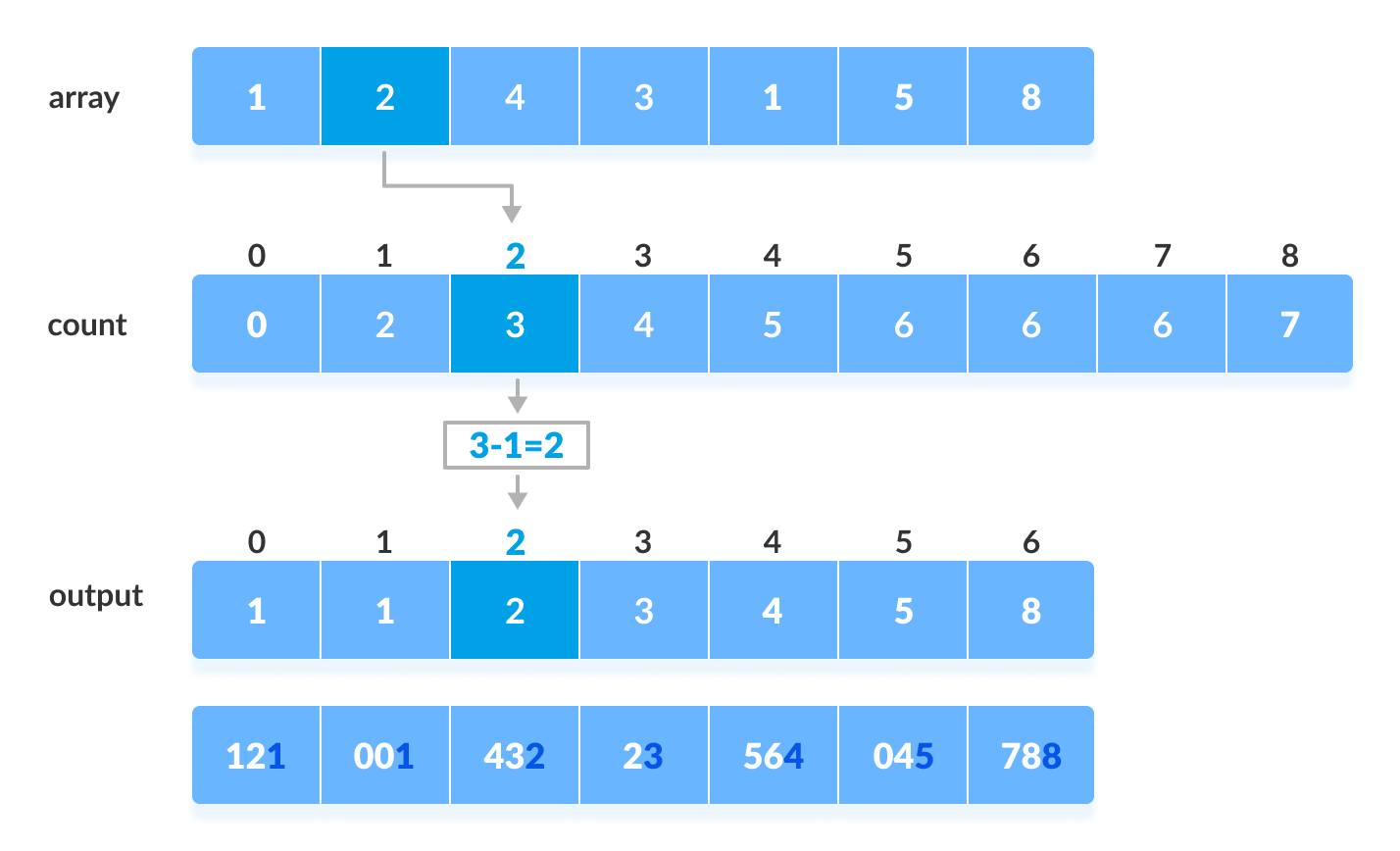
Digit by digit sort starting from least significant digit to most significant digit. Use counting sort to sort individual digits.
Steps:
For each digit i (least significant digit < i < most significant digit): sort input array using counting sort on the i’th digit

Radix sort is an integer sorting algorithm that sorts data with integer keys by grouping the keys by individual digits that share the same significant position and value (place value). Radix sort uses counting sort as a subroutine to sort an array of numbers. Because integers can be used to represent strings (by hashing the strings to integers), radix sort works on data types other than just integers. Because radix sort is not comparison based, it is not bounded by \Omega(n \log n)Ω(nlogn) for running time — in fact, radix sort can perform in linear time

# Using counting sort to sort the elements in the basis of significant places
def countingSort(array, place):
    size = len(array)
    output = [0] * size
    count = [0] * 10

    # Calculate count of elements
    for i in range(0, size):
        index = array[i] // place
        count[index % 10] += 1

    # Calculate cummulative count
    for i in range(1, 10):
        count[i] += count[i - 1]

    # Place the elements in sorted order
    i = size - 1
    while i >= 0:
        index = array[i] // place
        output[count[index % 10] - 1] = array[i]
        count[index % 10] -= 1
        i -= 1

    for i in range(0, size):
        array[i] = output[i]


# Main function to implement radix sort
def radixSort(array):
    # Get maximum element
    max_element = max(array)

    # Apply counting sort to sort elements based on place value.
    place = 1
    while max_element // place > 0:
        countingSort(array, place)
        place *= 10


data = [121, 432, 564, 23, 1, 45, 788]
radixSort(data)
print(data)

[1, 23, 45, 121, 432, 564, 788]

SEARCH ALGORITHMS

Interpolation search

Idea - return higher value of pos when searched value closer to arr[hi], and smaller when closer to arr[lo]
pos = lo + [ (x-arr[lo])*(hi-lo) / (arr[hi]-arr[Lo]) ]

On average the interpolation search makes about log(log(n)) comparisons (if the elements are uniformly distributed), where n is the number of elements to be searched. In the worst case (for instance where the numerical values of the keys increase exponentially) it can make up to O(n) comparisons

O(1) space complexity

Usage: improvement over Binary Search for instances, where the values in a sorted array are uniformly distributed. Binary goes to the middle while interpolation may go closer the element to be found. Formula for position:
pos = lo + [ (x-arr[lo])*(hi-lo) / (arr[hi]-arr[Lo]) ]

arr[] ==> Array where elements need to be searched
x ==> Element to be searched
lo ==> Starting index in arr[]
hi ==> Ending index in arr[]

# If x is present in arr[0..n-1], then returns 
# index of it, else returns -1 
def interpolationSearch(arr, n, x): 
    # Find indexs of two corners 
    lo = 0
    hi = (n - 1) 
   
    # Since array is sorted, an element present 
    # in array must be in range defined by corner 
    while lo <= hi and x >= arr[lo] and x <= arr[hi]: 
        if lo == hi: 
            if arr[lo] == x:  
                return lo; 
            return -1; 
          
        # Probing the position with keeping 
        # uniform distribution in mind. 
        pos  = lo + int(((float(hi - lo) / 
            ( arr[hi] - arr[lo])) * ( x - arr[lo]))) 
  
        # Condition of target found 
        if arr[pos] == x: 
            return pos 
   
        # If x is larger, x is in upper part 
        if arr[pos] < x: 
            lo = pos + 1; 
   
        # If x is smaller, x is in lower part 
        else: 
            hi = pos - 1; 
      
    return -1

# Driver Code 
# Array of items oin which search will be conducted 
arr = [10, 12, 13, 16, 18, 19, 20, 21, 22, 23, 24, 33, 35, 42, 47] 
n = len(arr) 
  
x = 18 # Element to be searched 
index = interpolationSearch(arr, n, x) 
  
if index != -1: 
    print("Element found at index", index) 
else: 
    print("Element not found")

Element found at index 4

Jump Search

• Time Complexity : O(√n)
• Auxiliary Space : O(1)

Like Binary Search, Jump Search is a searching algorithm for sorted arrays. The basic idea is to check fewer elements (than linear search) by jumping ahead by fixed steps or skipping some elements in place of searching all elements.

For example, suppose we have an array arr[] of size n and block (to be jumped) size m. Then we search at the indexes arr[0], arr[m], arr[2m]…..arr[km] and so on. Once we find the interval (arr[km] < x < arr[(k+1)m]), we perform a linear search operation from the index km to find the element x.

Let’s consider the following array: (0, 1, 1, 2, 3, 5, 8, 13, 21, 34, 55, 89, 144, 233, 377, 610). Length of the array is 16. Jump search will find the value of 55 with the following steps assuming that the block size to be jumped is 4. STEP 1: Jump from index 0 to index 4; STEP 2: Jump from index 4 to index 8; STEP 3: Jump from index 8 to index 12; STEP 4: Since the element at index 12 is greater than 55 we will jump back a step to come to index 8. STEP 5: Perform linear search from index 8 to get the element 55.

What is the optimal block size to be skipped? In the worst case, we have to do n/m jumps and if the last checked value is greater than the element to be searched for, we perform m-1 comparisons more for linear search. Therefore the total number of comparisons in the worst case will be ((n/m) + m-1). The value of the function ((n/m) + m-1) will be minimum when m = √n. Therefore, the best step size is m = √n.

Important points:

Works only sorted arrays. The optimal size of a block to be jumped is (√ n). This makes the time complexity of Jump Search O(√ n). The time complexity of Jump Search is between Linear Search ( ( O(n) ) and Binary Search ( O (Log n) ). Binary Search is better than Jump Search, but Jump search has an advantage that we traverse back only once (Binary Search may require up to O(Log n) jumps, consider a situation where the element to be searched is the smallest element or smaller than the smallest). So in a system where binary search is costly, we use Jump Search

import math

def jumpSearch( arr , x , n ): 
      
    # Finding block size to be jumped 
    step = math.sqrt(n) 
      
    # Finding the block where element is 
    # present (if it is present) 
    prev = 0
    while arr[int(min(step, n)-1)] < x: 
        prev = step 
        step += math.sqrt(n) 
        if prev >= n: 
            return -1
      
    # Doing a linear search for x in  
    # block beginning with prev. 
    while arr[int(prev)] < x: 
        prev += 1
          
        # If we reached next block or end  
        # of array, element is not present. 
        if prev == min(step, n): 
            return -1
      
    # If element is found 
    if arr[int(prev)] == x: 
        return prev 
      
    return -1

# Driver code to test function 
arr = [ 0, 1, 1, 2, 3, 5, 8, 13, 21, 
    34, 55, 89, 144, 233, 377, 610 ] 
x = 55
n = len(arr) 
  
# Find the index of 'x' using Jump Search 
index = jumpSearch(arr, x, n) 
  
# Print the index where 'x' is located 
print("Number" , x, "is at index" ,"%.0f"%index) 

Number 55 is at index 10

Exponential Search

Find range where element is present Do Binary Search in above found range. How to find the range where element may be present? The idea is to start with subarray size 1, compare its last element with x, then try size 2, then 4 and so on until last element of a subarray is not greater. Once we find an index i (after repeated doubling of i), we know that the element must be present between i/2 and i (Why i/2? because we could not find a greater value in previous iteration)

Time Complexity : O(Log n) Auxiliary Space : The above implementation of Binary Search is recursive and requires O(Log n) space. With iterative Binary Search, we need only O(1) space.

Applications of Exponential Search:

Exponential Binary Search is particularly useful for unbounded searches, where size of array is infinite. Please refer Unbounded Binary Search for an example. It works better than Binary Search for bounded arrays, and also when the element to be searched is closer to the first element.

# Returns the position of first 
# occurrence of x in array 
def exponentialSearch(arr, n, x): 
    # IF x is present at first  
    # location itself 
    if arr[0] == x: 
        return 0
          
    # Find range for binary search  
    # j by repeated doubling 
    i = 1
    while i < n and arr[i] <= x: 
        i = i * 2
      
    # Call binary search for the found range 
    return binarySearch( arr, i / 2,  
                         min(i, n), x)

# Driver Code 
arr = [2, 3, 4, 10, 40] 
n = len(arr) 
x = 10
result = exponentialSearch(arr, n, x) 
if result == -1: 
    print "Element not found in thye array"
else: 
    print "Element is present at index %d" %(result) 

Binary vs. Linear

• Input data needs to be sorted in Binary Search and not in Linear Search
• Linear search does the sequential access whereas Binary search access data randomly.
• Time complexity of linear search - O(n) , Binary search has time complexity O(log n).
• Linear search performs equality comparisons and Binary search performs ordering comparisons

Binary search does less comparisons than tertiary

The following is recursive formula for counting comparisons in worst case of Binary Search.

T(n) = T(n/2) + 2, T(1) = 1 The following is recursive formula for counting comparisons in worst case of Ternary Search.

T(n) = T(n/3) + 4, T(1) = 1 In binary search, there are 2Log2n + 1 comparisons in worst case. In ternary search, there are 4Log3n + 1 comparisons in worst case.

Time Complexity for Binary search = 2clog2n + O(1) Time Complexity for Ternary search = 4clog3n + O(1) Therefore, the comparison of Ternary and Binary Searches boils down the comparison of expressions 2Log3n and Log2n . The value of 2Log3n can be written as (2 / Log23) * Log2n . Since the value of (2 / Log23) is more than one, Ternary Search does more comparisons than Binary Search in worst case

Selection Sort

Based on https://github.com/agnedil/Code-Python-Algorithms-Notebooks/blob/master/ipython_nbs/sorting/selection_sort.ipynb

• One of the simplest and classic sorting algorithms.
• Complexity of O(n^2) (list of n elements is sorted n times).
• In-place sorting of an array:
• Find the smallest element in $[array[1] : array[n]]$ and swap it with array[0] if it is < $array[0]$;
• Repeat the same, but for $array[n-1]$, swapping with $array[1]$, and so on.
• First iteration checks n elements, second iteration checks n-1 elements, third - n-2, and so forth => # of checks is $n\times 1/2 \times n$. But Big O omits constants => $O(n^2)$ instead of $O(n\times 1/2 \times n)$.

# sorting f(x)
def selection_sort(myarr):
    
    # iterate over the array
    for i in range (len(myarr)-1):
        min_idx = i + 1
        
        # find the smallest element on the right excluding the leftmost element
        for j in range(i + 2, len(myarr)):
            if myarr[j] < myarr[min_idx]:
                min_idx = j
                
        # compare the smallest element found on the right w/the leftmost element and swap if smaller
        if myarr[min_idx] < myarr[i]:
            myarr[min_idx], myarr[i] = myarr[i], myarr[min_idx]
            
    return myarr

# test sorting f(x)
a, b, c, d = [8, 7, 4, 2, 1, 25, 29, 38, 45, 5, 101, 97, 73, 74, 72, 55], [8, 7, 4, 2, 1], [8, 7, 2, 11], [8, 7]
for arr in [a, b, c, d]:
    print(arr, end=' ')
    print('=> ', merge_sort(arr))

[8, 7, 4, 2, 1, 25, 29, 38, 45, 5, 101, 97, 73, 74, 72, 55] =>  [1, 2, 4, 5, 7, 8, 25, 29, 38, 45, 55, 72, 73, 74, 97, 101]
[8, 7, 4, 2, 1] =>  [1, 2, 4, 7, 8]
[8, 7, 2, 11] =>  [2, 7, 8, 11]
[8, 7] =>  [7, 8]

Edit Levenshtein Distance (another solution)

https://stackoverflow.com/questions/2460177/edit-distance-in-python https://en.wikibooks.org/wiki/Algorithm_Implementation/Strings/Levenshtein_distance#Python

# wiki
def levenshtein(s1, s2):
    if len(s1) < len(s2):
        return levenshtein(s2, s1)

    # len(s1) >= len(s2)
    if len(s2) == 0:
        return len(s1)

    previous_row = range(len(s2) + 1)
    for i, c1 in enumerate(s1):
        current_row = [i + 1]
        for j, c2 in enumerate(s2):
            insertions    = previous_row[j + 1] + 1       # j+1 instead of j since previous_row and current_row are one char longer            
            substitutions = previous_row[j] + (c1 != c2)
            deletions     = current_row[j] + 1             # than s2
            current_row.append(min(insertions, deletions, substitutions))
        previous_row = current_row
        print(previous_row)
    
    return previous_row[-1]

levenshtein('aborigenous', 'sc')

[1, 1, 2]
[2, 2, 2]
[3, 3, 3]
[4, 4, 4]
[5, 5, 5]
[6, 6, 6]
[7, 7, 7]
[8, 8, 8]
[9, 9, 9]
[10, 10, 10]
[11, 10, 11]
11