GRAPH REPRESENTATION AND TRAVERSALS
Complete list of graph algos at middle of page here and selected algos (most covered here) at end of Content here
Graphs can represent systems of roads, airline flights from city to city, Internet connections, sequence of classes for a computer science degree. Once we have a good representation for a problem - we can use standard graph algorithms to solve it. Trees are just a special kind of graph.
Graphs have: * vertices / nodes that can have names (keys) and payloads (additional info); * edges each connecting a pair of vertices (relationships); unordered pairs of verticies - undirected graph; ordered vertices: directed graph / digraph; * weights on edges - cost to go from one vertex to another (distance between cities in a graph of roads).
Path - sequence of vertices connected by edges. Path = w_1, w_2, ..., w_n, such that (w_i, w_{i+1}) ∈E for all i in 1 <= i <= n−1. Path length - # edges in unweighted g. (n−1) OR sum of the weights in weighted g.
Cycle in directed graph - path that starts and ends at the same vertex. If no cycles - acyclic graph; if also directed - directed acyclic graph (DAG).
GRAPHS VS. TREES
Graph - collection of two sets: finite non-empty set of vertices v and finite non-empty set of edges e. * Vertices are nothing but the nodes in the graph. * Two adjacent vertices are joined by edges. * Any graph is denoted as G = {V, E}.
Tree - finite set of one or more nodes such that * There is a root Node; * The remaining nodes are partitioned into n>=0 disjoint sets T1, T2, T3, …, Tn of subtrees of root.
G. = non-linear data structure.
T. = non-linear data structure.
G. = collection of vertices/nodes and edges.
T. = collection of nodes and edges.
G. - each node can have any # edges.
T. - in general, each node can have any number of child nodes, but binary trees - two at the most.
G. - no unique root node
T. - unique root node
G. - can have cycles
T. - no cycles
G. - used for finding shortest path
T. - used for game trees, decision trees
Graph Representations - Pros and Cons
Factors to consider:
Time and space complexity (c.)
Data sparseness
* Choose representation depending on algo and # nodes
Adjacency matrix representation (r.)
2D array (matrix) of size n×n for a graph with n vertices. Each cell [i, j] indicates whether there is an edge between vertex i and vertex j (if edge - value is 1 or the weight, and 0 if no edge).
    0  1  2  3
0 [ 0, 1, 1, 0 ]
1 [ 1, 0, 1, 0 ]
2 [ 1, 1, 0, 1 ]
3 [ 0, 0, 1, 0 ]
Pros * Quick Edge Lookup: O(1) time - simple [i, j] index lookup to see if edge present, add / remove edge. * Simplicity: The matrix is straightforward to understand and implement. Matrix operations can get you insights into nature of graph, relationships between its vertices and makes many problems easier (algebraic graph theory: kth power of the adjacency matrix - # paths of length k from vertex i to vertex j, add identity matrix before taking the kth power to get # paths of length <=k, take a rank n-1 minor of the Laplacian to get # spanning trees), but at the expense of space complexity; * Using matrix saves from allocating extra pointers (word size in memory)
Cons
* Memory Intensive: O(n²) space - space c. O(n^2) => good for dense graphs, inefficient for sparse graphs, and graphs usually don't have too many connections => adjacency lists are better for most tasks.
* Inefficient Iteration: O(n) to get a vertex's adjacency list (n = # verticies) because have to look through every cell in a row, even if a small # vertices are adjacent - many are 0 (or “no edge”); inEdges (list of incoming edges) and outEdges are time expensive too; O(V^2) add vertex.
Other * better for graphs with weighted edges (object/pointer r. stores edge weights in a || array to be synchronized with pointer array); * Undirected graphs - adjacency matrix is symmetric
Adjacency list r.
Array (or dict) where each index (key) corresponds to a vertex, and the value is a list of all adjacent vertices (neighbors). For weighted graphs, these lists can include the weights along with the vertex identifiers.
0: [1, 2]
1: [0, 2]
2: [0, 1, 3]
3: [2]
Pros * Space Efficient: O(V+E) OR O(2E) space c., stores only edges = connected vertices, no 0s, ideal for sparse graphs (E much < n²). * Efficient Neighbor Iteration: iterate over actual neighbors, no seros. time c. O(1) get a vertex's adjacency list (array indexing). * Flexibility: Easier to add or remove vertices and edges dynamically.
Cons * Slower Edge Lookup: O(n) (n=# vertices) see if edge (i,j) exists = get i's adjacency list in constant time + look for j in it - time complexity O(d) where d is the degree of node i which can be up to |V|-1. * Very dense graphs - overhead of maintaining lists for each vertex might not offer a significant benefit over an adjacency matrix.
Objects/pointer r.
* time c. O(n) access a node;
* space c. O(n) for obj. (# objects = # nodes); O(n^2) for pointers (to obj.) - each node may have pointers to up to n nodes;
* better for directed graphs than undirected (pointers to be maintained in pairs, which can become unsynchronized);
* have high search time c., but are natural for BST (a lot of extra structure)
More + correct names for the three r. methods here
Incidence matrix
2D Boolean matrix, rows = vertices, columns = edges, entries = is vertex incident to edge
Edge list
- = array of edges, edge = array of two vertex numbers (obj.) that edge is incident on. If weights - add third element to array or more info to obj.
- Simple, but time c. to find edge = O(E) if edge list unordered, but O(lgE) is desired
- Space c. Θ(E)
graph_as_edge_list = [ [0,1], [0,6], [0,8], [1,4], [1,6], [1,9], [2,4], [2,6], [3,4], [3,5],
[3,8], [4,5], [4,9], [7,8], [7,9] ]
Adjacency matrix
# Simple matrix (1s indicate that there is an edge, but it's possible to use weights instead of 1s)
graph_simple_adjacency_matrix = [
  [0, 1, 0, 0, 0, 0, 1, 0, 1, 0],
  [1, 0, 0, 0, 1, 0, 1, 0, 0, 1],
  [0, 0, 0, 0, 1, 0, 1, 0, 0, 0],
  [0, 0, 0, 0, 1, 1, 0, 0, 1, 0],
  [0, 1, 1, 1, 0, 1, 0, 0, 0, 1],
  [0, 0, 0, 1, 1, 0, 0, 0, 0, 0],
  [1, 1, 1, 0, 0, 0, 0, 0, 0, 0],
  [0, 0, 0, 0, 0, 0, 0, 0, 1, 1],
  [1, 0, 0, 1, 0, 0, 0, 1, 0, 0],
  [0, 1, 0, 0, 1, 0, 0, 1, 0, 0]
]
# https://www.programiz.com/dsa/graph-adjacency-matrix
class Graph(object):

    # Initialize the matrix
    def __init__(self, size):
        self.adjMatrix = []
        for i in range(size):
            self.adjMatrix.append([0 for i in range(size)])
        self.size = size

    # Add edges
    def add_edge(self, v1, v2):
        if v1 == v2:
            print("Same vertex %d and %d" % (v1, v2))
        self.adjMatrix[v1][v2] = 1
        self.adjMatrix[v2][v1] = 1

    # Remove edges
    def remove_edge(self, v1, v2):
        if self.adjMatrix[v1][v2] == 0:
            print("No edge between %d and %d" % (v1, v2))
            return
        self.adjMatrix[v1][v2] = 0
        self.adjMatrix[v2][v1] = 0

    def __len__(self):
        return self.size

    # Print the matrix
    def print_matrix(self):
        for row in self.adjMatrix:
            for val in row:
                print('{:4}'.format(val), end=' '),
            print()


def main():
    g = Graph(5)
    g.add_edge(0, 1)
    g.add_edge(0, 2)
    g.add_edge(1, 2)
    g.add_edge(2, 0)
    g.add_edge(2, 3)

    g.print_matrix()


if __name__ == '__main__':
    main()
   0    1    1    0    0
   1    0    1    0    0
   1    1    0    1    0
   0    0    1    0    0
   0    0    0    0    0
Adjacency list
# List of lists (set of sets), unweighted g.: ABC (012)
graph_list = [
  [1, 2],
  [0, 2],
  [0, 1],
  ]
# Dict of lists/sets, unweighted g.: ABC
graph_dict_unweighted = {
         'A': ['B', 'C'],
         'B': ['A', 'C'],
         'C': ['A', 'B']
}
# Dict of dicts, weighted g.: ABC
graph_dict_weighted = {
    'A': {'B':5, 'C':2},
    'B': {'A':3, 'C':4},
    'C': {'A':2, 'B':3}
}
There is one more complex representation as an adj list in which each element is a linked list - https://www.programiz.com/dsa/graph-adjacency-list. But this way, arrows inside each adj list don't mean that these two nodes are connected; they actually don't mean anything - counterintuitive!
# Directed graph as adjacency list
class Graph:

    def __init__(self):
        self.graph = dict()

    # add edge
    def addEdge(self, u, v):
        if u in self.graph:
            self.graph[u].add(v)
        else:
            self.graph[u] = set([v])

g = Graph()
g.addEdge(0, 1)
g.addEdge(0, 2)
g.addEdge(1, 2)
g.addEdge(2, 0)
g.addEdge(2, 3)
g.addEdge(3, 3)

print('Printing graph:')
for k, v in g.graph.items():
    print(k, v)
Printing graph:
0 {1, 2}
1 {2}
2 {0, 3}
3 {3}
To make the above undirected, add each pair of vertices twice: first as (0,1) then as (1,0)
Depth First Search (DFS)
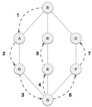
Rules:
* Rule 1 − Visit the adjacent unvisited vertex. Mark it as visited. Display it. Push it in a stack.
* Rule 2 − If no adjacent vertex is found, pop up a vertex from the stack. (It will pop up all the vertices from the stack, which do not have adjacent vertices.)
* Rule 3 − Repeat Rule 1 and Rule 2 until the stack is empty.
More: Great graph DFT & BFT visuals and sequence of rules to follow and here too
Rules (short): * Mark the current vertex as being visited. * Explore each adjacent vertex that is not included in the visited set
every edge is considered exactly twice, and every node is processed exactly once, so the complexity has to be a constant multiple of the number of edges and the number of vertices
time complexity = (V + E), where V is # nodes and E is # edges;
space complexity = O(V)
Applications:
* To build index by search index
* For GPS navigation
* Path finding algorithms
* In Ford-Fulkerson algorithm to find maximum flow in a network
* Cycle detection in an undirected graph
* In minimum spanning tree
# Udemy iterative
def dfs1(graph, start):

    visited, stack = set(), [start]

    while stack:
        vertex = stack.pop()
        if vertex not in visited:
            print(vertex, end=' ')
            visited.add(vertex)
            stack.extend(graph[vertex] - visited)

    return visited

graph = { 0: set([1, 2]),
          1: set([2]),
          2: set([3]),
          3: set([1, 2])
        }
dfs1(graph, 0)
0 2 3 1 {0, 1, 2, 3}# Recursive: https://www.programiz.com/dsa/graph-dfs (BETTER THAN GFG) + Udemy def dfs2(graph, start, visited=None): if visited is None: visited = set() visited.add(start) print(start) for next in graph[start] - visited: dfs2(graph, next, visited) return visited graph = {'0': set(['1', '2']), '1': set(['0', '3', '4']), '2': set(['0']), '3': set(['1']), '4': set(['2', '3'])} dfs2(graph, '0')
0
1
3
4
2
2
{'0', '1', '2', '3', '4'}
Breadth First Search (BFS)
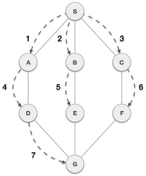
It finds all the vertices that are a distance k from s before it finds any vertices that are a distance k+1
Rules:
* Rule 1 − Visit the adjacent unvisited vertex. Mark it as visited. Display it. Insert it in a queue.
* Rule 2 − If no adjacent vertex is found, remove the first vertex from the queue.
* Rule 3 − Repeat Rule 1 and Rule 2 until the queue is empty.
More: Great graph DFT & BFT visuals and sequence of rules to follow and here too
time complexity = (V + E), where V is # nodes and E is # edges;
space complexity = O(V)
Applications:
* find path
* test if graph is bipartite
* find strongly connected components
* detect cycles
# Udemy iterative
def bfs(graph, start):

    visited = set()
    queue   = [start]

    while queue:
        vertex = queue.pop(0)
        if vertex not in visited:
            print(vertex, end = ' ')
            visited.add(vertex)
            queue.extend(graph[vertex] - visited)

    return visited

graph = {0: set([1, 2]), 1: set([2]), 2: set([3]), 3: set([1, 2])}
bfs(graph, 0)
0 1 2 3 {0, 1, 2, 3}def bfs2(graph, start): ''' Leetcode ''' visited, queue = {start}, [start] while queue: vertex = queue.pop(0) print(str(vertex) + " ", end="") for neighbor in graph[vertex]: if neighbor not in visited: visited.add(neighbor) queue.append(neighbor) graph = {0: [1, 2], 1: [2], 2: [3], 3: [1, 2]} print('BFS:') bfs2(graph, 0) graph = {0: set([1, 2]), 1: set([2]), 2: set([3]), 3: set([1, 2])} print('\nBFS:') bfs2(graph, 0)
BFS:
0 1 2 3
BFS:
0 1 2 3
All Paths from Vertex A to Vertex B
Udemy
The implementation below uses the stack data-structure again to iteratively solve the problem, yielding each possible path when we locate the goal. Using a generator allows the user to only compute the desired amount of alternative paths.
def dfs_paths(graph, start, goal):

    stack = [(start, [start])]

    while stack:
        (vertex, path) = stack.pop()
        for nxt in graph[vertex] - set(path):
            if nxt == goal:
                yield path + [nxt]
            else:
                stack.append((nxt, path + [nxt]))
def bfs_paths(graph, start, goal):
    queue = [(start, [start])]
    while queue:
        (vertex, path) = queue.pop(0)
        for nxt in graph[vertex] - set(path):
            if nxt == goal:
                yield path + [nxt]
            else:
                queue.append((nxt, path + [nxt]))
graph = {'A': set(['B', 'C']),
         'B': set(['A', 'D', 'E']),
         'C': set(['A', 'F']),
         'D': set(['B']),
         'E': set(['B', 'F']),
         'F': set(['C', 'E'])}

list(bfs_paths(graph, 'A', 'F'))
[['A', 'C', 'F'], ['A', 'B', 'E', 'F']]
Shortest path using bfs all paths algo
Knowing that the shortest path will be returned first from the BFS path generator method we can create a useful method which simply returns the shortest path found or ‘None’ if no path exists. As we are using a generator this in theory should provide similar performance results as just breaking out and returning the first matching path in the BFS implementation.
def shortest_path(graph, start, goal):
    try:
        return next(bfs_paths(graph, start, goal))
    except StopIteration:
        return None

shortest_path(graph, 'A', 'F')
['A', 'C', 'F']
Topological Sorting
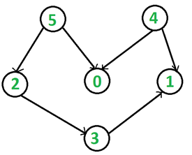
Possible only for Directed Acyclic Graph (DAG) - linear ordering of vertices such that for every directed edge uv, vertex u comes before v in the ordering. There can be more than one topological sorting for a graph. The first vertex in topological sorting is always a vertex with in-degree 0 (a vertex with no incoming edges).
For example, a topological sorting of the following graph is “5 4 2 3 1 0”; another topological sorting of the following graph is “4 5 2 3 1 0”.
# source: https://algocoding.wordpress.com/2015/04/05/topological-sorting-python/
# Notation: k = node as key, v = node as value inside adjancy list
# Three vars:
# 1) in_degree    =  DICT { node : in-degree }
# 2) q            =  LIST of nodes with 0 in-degree
#                         (when a node is popped from it, in-degree of nodes from its adj. list decreases by 1)
# 3) topo_sorted  =  LIST of sorted nodes (result)

def kahn_toposort( graph ):

    topo_sorted = []                                              # sorted nodes

    in_degree = { k: 0 for k in graph }                           # get in-degree of each node
    for k in graph:
        for v in graph[ k ]:
            in_degree[v] += 1

    q = [ k for k,v in in_degree.items() if v == 0 ]              # nodes with 0 in-degree
    while q:
        k = q.pop()                                               # remove 1 node w/0 in-degree
        topo_sorted.append( k )
        for v in graph[ k ]:                                      # decrease in-degree its adjacent vertices
            in_degree[ v ] -= 1
            if in_degree[ v ] == 0:                               # keep track if any other node reaches 0
                q.append( v )

    return topo_sorted if len(topo_sorted) == len(graph) else []          # no topo_sort if there is a cycle


tasks =       { "have lunch" : ["wash the dishes"],
                "cook food" : ["have lunch", "wash the dishes"],
                "wash laundry" : ["dry laundry", "fold laundry"],
                "dry laundry" : ["fold laundry"],
                "fold laundry" : ["cook food"],
                "wash the dishes": ["watch TV"],
                "watch TV": [],
              }

kahn_toposort( tasks )
['wash laundry',
 'dry laundry',
 'fold laundry',
 'cook food',
 'have lunch',
 'wash the dishes',
 'watch TV']
Shortest Path with Dijkstra’s Algorithm
Time = O(V + E * log E)
DESCRIPTION: https://bradfieldcs.com/algos/graphs/dijkstras-algorithm/
Iterative algo to find shortest path from one node to all other nodes in the graph (~BFS).
- Distances dict - to keep track of total cost FROM start node TO each destination; initialize w/0 for start node, and inf for rest.
- Update these values until they represent the smallest weight path FROM start TO each destination.
The order in which we iterate over vertices is controlled by a priority queue (heapq module) with tuples (distance, vertex) - maintains sorting by distance. This ensures that as we explore one vertex after another, we are always exploring the one with the smallest distance
heapq lib = min heap, zero-based
initialize                 - heap = heapq.heapify( my_list )
heap[0]                    - min elem
heap.sort()                - maintains the heap invariant
heapq.heappush(heap, item) - push item onto heap, maintaining heap invariant
heapq.heappop(heap)        - pop and return smallest item from heap, maintaining the heap invariant. To access the smallest item without popping - heap[0]. IndexError if heap empty
import heapq    # min heap (a.k.a. priority queue)


def calculate_distances(graph, starting_vertex):

    distances = {vertex: float('infinity') for vertex in graph}
    distances[starting_vertex] = 0
    pq = [(0, starting_vertex)]

    while len(pq) > 0:

        current_distance, current_vertex = heapq.heappop(pq)

        # Nodes can get added to pq multiple times. We process vertex first time it's removed from pq
        if current_distance > distances[current_vertex]:
            continue

        for neighbor, weight in graph[current_vertex].items():
            distance = current_distance + weight

            # Only consider new path if it's better than before
            if distance < distances[neighbor]:
                distances[neighbor] = distance
                heapq.heappush(pq, (distance, neighbor))

    return distances


example_graph = {
    'U': {'V': 2, 'W': 5, 'X': 1},
    'V': {'U': 2, 'X': 2, 'W': 3},
    'W': {'V': 3, 'U': 5, 'X': 3, 'Y': 1, 'Z': 5},
    'X': {'U': 1, 'V': 2, 'W': 3, 'Y': 1},
    'Y': {'X': 1, 'W': 1, 'Z': 1},
    'Z': {'W': 5, 'Y': 1},
}
print(calculate_distances(example_graph, 'X'))
{'U': 1, 'V': 2, 'W': 2, 'X': 0, 'Y': 1, 'Z': 2}Comparison of Dijkstra’s and Floyd–Warshall algorithms
Main Purposes: * Dijkstra’s Algorithm is one example of a single-source shortest algorithm (SSSP), i.e. it finds shortest path from a source vertex to all other vertices. * Floyd Warshall Algorithm is an example of all-pairs shortest path algorithm, meaning it computes the shortest path between all pair of nodes.
Time Complexities : * Dijkstra’s Algorithm: O(E log V) * Floyd Warshall: O(V3)
Other Points: * We can use Dijskstra’s shortest path algorithm for finding all pair shortest paths by running it for every vertex. But time complexity of this would be O(VE Log V) which can go (V3 Log V) in worst case. * Another important differentiating factor between the algorithms is their working towards distributed systems. Unlike Dijkstra’s algorithm, Floyd Warshall can be implemented in a distributed system, making it suitable for data structures such as Graph of Graphs (Used in Maps). * Lastly Floyd Warshall works for negative edge (but not negative cycle), whereas Dijkstra’s algorithm not.
Note: negative cycle - overall sum of cycle is negative
Floyd Warshall Algorithm
Time c. O(V^3)
# all-pair shortest paths
def floyd_warshall(graph):

    """ dist[][] - output matrix of shortest distances between all pair of vertices
        When initialized - it contains shortest paths considering no intermediate vertices
    """

    dist = list(map(lambda i : list(map(lambda j : j , i)) , graph))

    for k in range(V):

        for i in range(V):                                                               # all vertices as source

            for j in range(V):                                                           # all vertices as destination

                # update dist[i][j] if vertex k on shortest path from i to j
                dist[i][j] = min(dist[i][j], dist[i][k] + dist[k][j])

    printSolution(dist)


# A utility function to print the solution
def printSolution(dist):

    print('Shortest distances:')
    for i in range(V):
        for j in range(V):
            if(dist[i][j] == INF):
                print('INF', end=' ')
            else:
                print(dist[i][j], end=' ')
            if j == V-1:
                print('')


# Create this weighted graph
# Note how path 0 -> 3 is not selected because it's not the shortest path (weight 10)
"""
            10
       (0)------->(3)
        |         /|\
      5 |          |
        |          | 1
       \|/         |
       (1)------->(2)
            3
"""


# used for unconnected vertices
INF  = 99999

graph = [[0,    5,  INF,  10],
         [INF,  0,   3,   INF],
         [INF, INF,  0,    1],
         [INF, INF, INF,   0]
        ]

# number of vertices in graph
V = len(graph)

floyd_warshall(graph)
Shortest distances:
0 5 8 9
INF 0 3 4
INF INF 0 1
INF INF INF 0
Articulation points in a graph
In an undirected connected graph, a vertex is an articulation point (cut vertex) iff removing it with its edges disconnects the graph.
In an undirected disconnected graph, a vertex is an articulation point iff removing it increases number of disconnected components.
Articulation points are vulnerabilities – single points whose failure would split the network into 2 or more components.
Algorithm to find articulation points
For every vertex v:
a) Remove v from graph
b) See if the graph remains connected (We can either use BFS or DFS)
c) Add v back to the graph
Bridges in a graph
In an undirected connected graph, an edge is a bridge iff removing it disconnects the graph.
In an undirected disconnected graph, an edge is a bridge iff removing it increases number of disconnected components.
Articulation points and bridges are vulnerabilities in a connected network; useful for designing reliable networks. Example: in a wired computer network, an articulation point is a critical computers and a bridge is a critical connection.
Algorithm to find bridges
For every edge (u, v):
a) Remove (u, v) from graph
b) See if the graph remains connected (using BFS or DFS)
c) Add (u, v) back to the graph
Strongly connected component,
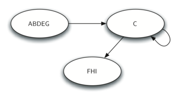
C, of a graph G, as the largest subset of vertices C⊂V such that for every pair of vertices v,w∈C we have a path from v to w and a path from w to v. Figure below - three strongly connected components (different shades). Algo = DFS
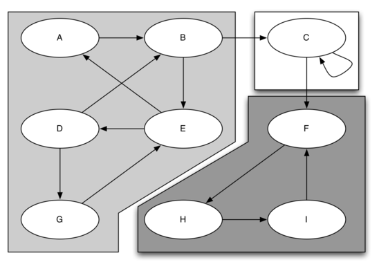
Once the strongly connected components have been identified we can show a simplified view of the graph by combining all the vertices in one strongly connected component into a single larger vertex. The simplified version of the graph above is shown below
Minimum Spanning Tree - Prim's Algo
S.t. for a graph G = (V,E) is acyclic subset of E connecting all vertices in V (sum of edge weights in T is minimized)
Used for most efficient transfer of information to every listener (in gaming - for all players to know latest position of other players; in Internet radio for all listeners to fully reconstruct current song). There may be several spanning trees - we need to find the minimum one.
Similar to Dijkstra’s algo, Prim’s algo uses a priority queue to select next vertex to add to growing graph
from collections import defaultdict
import heapq


def create_spanning_tree(graph, start):

    mst     = defaultdict(set)
    visited = set([ start ])
    edges   = [
                (cost, start, to)
                for to, cost in graph[start].items()
              ]
    heapq.heapify(edges)

    while edges:
        cost, frm, to = heapq.heappop(edges)
        if to not in visited:
            visited.add(to)
            mst[frm].add(to)
            for to_next, cost in graph[to].items():
                if to_next not in visited:
                    heapq.heappush(edges, (cost, to, to_next))

    return mst

example_graph = {
    'A': {'B': 2, 'C': 3},
    'B': {'A': 2, 'C': 1, 'D': 1, 'E': 4},
    'C': {'A': 3, 'B': 1, 'F': 5},
    'D': {'B': 1, 'E': 1},
    'E': {'B': 4, 'D': 1, 'F': 1},
    'F': {'C': 5, 'E': 1, 'G': 1},
    'G': {'F': 1},
}

dict(create_spanning_tree(example_graph, 'A'))
{'A': {'B'}, 'B': {'C', 'D'}, 'D': {'E'}, 'E': {'F'}, 'F': {'G'}}Graph algos (find Python): https://www.programiz.com/dsa/spanning-tree-and-minimum-spanning-tree, https://www.programiz.com/dsa/bellman-ford-algorithm, https://www.programiz.com/dsa/dijkstra-algorithm + other links on the same page
TREE REPRESENTATIONS AND TRAVERSALS
https://bradfieldcs.com/algos/trees/representing-a-tree/
https://pythonspot.com/python-tree/
http://www.cs.utsa.edu/~wagner/python/tree.lists/trees.html
TYPES OF TREES:
* m-ary tree (k-ary or k-way tree) - rooted tree in graph theory in which each node has no more than m children (m = 2 is binary, m = 3 is ternary). Note: rooted means there is a root
* Binary tree (BT) - each node has at most two children
* Complete BT = binary tree in which every level is completely filled, except possibly the last, and all nodes are as far left as possible.
* BST - parent's value greater that values in left subtree & less values in right subtree
* Binary Heap (max or min heap) = Complete Binary Tree such that: parent's value greater (or smaller) than values in children. Array repr. - space efficient: if node's index = i, node's parent = (i-1)/2, left child = 2 * i + 1, right child = 2 * i + 2, (0-based).
* Full (proper or plane) BT - every node has 0 or 2 children
* Perfect BT - all interior nodes have two children and all leaves have the same depth (level)
* Infinite complete BT - every node has two children (set of levels is infinite)
* Balanced BT - left and right subtrees of every node differ in height by no more than 1
* Degenerate (pathological) tree - each parent has only one child = linked list
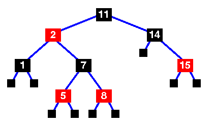
THEORY * Red–black tree is a kind of self-balancing BST. Each node stores an extra bit representing color, used to ensure that the tree remains approximately balanced during insertions and deletions. Rules:
- Every node is either red or black.
- Every leaf (NULL) is black.
- If a node is red, then both its children are black.
- Every simple path from a node to a descendant leaf contains the same number of black nodes
 Lemma
Lemma
A red-black tree with n internal nodes has height at most 2log(n+1) - RBTs are good for search: can always be searched in O(log n) time (insertions and deletions too while usually it's O(h) or even O(n) for imbalanced tree)
-
Randomized quicksort: random number to pick next random pivot (or shuffle the array).
randpivot = random.randrange(start, stop) -
Minimum cut - min subset of edges that, when removed, disconnects [undirected, weighted] graph. Application: in communications, nodes of the cut are critical for network integrity
-
Spanning tree - subgraph (tree) of undirected graph that includes ALL VERTICES & MIN # EDGES (can be several, but min. s. t. = min. sum of weights)
1. TREE REPRESENTATION (object, list, dictionary)
1a. OBJECT
# Node as class
class Node:
    def __init__(self, val):
        self.val = val
        self.left = None
        self.right = None

    def insert_left(self, child):
        if self.left is None:
            self.left = child
        else:
            child.left = self.left
            self.left = child

    def insert_right(self, child):
        if self.right is None:
            self.right = child
        else:
            child.right = self.right
            self.right = child
# NO NEED TO EVEN USE INSERT FUNCTIONS!
root = Node('a')
print(root.val)
print(root.left)

root.left = Node('b')
print(root.left)
print(root.left.val)

root.right = Node('c')
print(root.right)
print(root.right.val)

root.right.val = 'hello'
print(root.right.val)
a
None
<__main__.Node object at 0x000001AFEF9F4C88>
b
<__main__.Node object at 0x000001AFEF9F41D0>
c
hello
# USING THE INSERT FUNCTIONS
root = Node('a')
print(root.val)  # => 'a'
print(root.left)  # => None

root.insert_left(Node('b'))
print(root.left)  # => <__main__.Node object>
print(root.left.val)  # => 'b'

root.insert_right(Node('c'))
print(root.right)  # => <__main__.Node object>
print(root.right.val)  # => 'c'

root.right.val = 'hello'
print(root.right.val)  # => 'hello'
a
None
<__main__.Node object at 0x000001AFEF9F41D0>
b
<__main__.Node object at 0x000001AFEF9F4EB8>
c
hello
1b. LIST
This generalizes to a tree that has many subtrees (more than binary tree) - another subtree is just another list
# LIST
tree = [
    'a',  #root
    [
        'b',  # left subtree
        ['d' [], []],
        ['e' [], []]
    ],
    [
        'c',  # right subtree
        ['f' [], []],
        []
    ]
]
tree = ['a', ['b', ['d', [], []], ['e', [], []]], ['c', ['f', [], []], []]]

# the root
print(tree[0])  # => 'a'

# the left subtree
print(tree[1])  # => ['b', ['d', [], []], ['e', [], []]]

# the right subtree
print(tree[2])  # => ['c', ['f', [], []], []]
['b', ['d', [], []], ['e', [], []]]
['c', ['f', [], []], []]
a
To add left subtree to root - insert new list into second position of root list. Careful: if the list already has something in the second position - keep track of it and push it down the tree as left child of list being added
def BinaryTree(r):
    return [r, [], []]

def insert_left(root, child_val):
    subtree = root.pop(1)
    if len(subtree) > 1:
        root.insert(1, [child_val, subtree, []])
    else:
        root.insert(1, [child_val, [], []])
    return root

def insert_right(root, child_val):
    subtree = root.pop(2)
    if len(subtree) > 1:
        root.insert(2, [child_val, [], subtree])
    else:
        root.insert(2, [child_val, [], []])
    return root

# abstract away the use of positions in list to represent tree, left subtrees and right subtrees
def get_root_val(root):
    return root[0]

def set_root_val(root, new_val):
    root[0] = new_val

def get_left_child(root):
    return root[1]

def get_right_child(root):
    return root[2]
root = [3, [], []]
insert_left(root, 4)
insert_left(root, 5)
insert_right(root, 6)
insert_right(root, 7)
left = get_left_child(root)
print(left)  # => [5, [4, [], []], []]

set_root_val(left, 9)
print(root)  # => [3, [9, [4, [], []], []], [7, [], [6, [], []]]]

insert_left(left, 11)
print(root)  # => [3, [9, [11, [4, [], []], []], []], [7, [], [6, [], []]]]
print(get_right_child(get_right_child(root)))  # => [6, [], []]
[5, [4, [], []], []]
[3, [9, [4, [], []], []], [7, [], [6, [], []]]]
[3, [9, [11, [4, [], []], []], []], [7, [], [6, [], []]]]
[6, [], []]
1c. MAP (DICTIONARY)
- PROs of list representation: succinct, easily construct, serialize and print trees, portable to languages and contexts without objects.
- CONs: difficult to see the tree-like nature of the composite lists.
Therefore, using a very similar representation with nested mappings (dicts) is preferred in practice + we can name children, values and potentially other data in a node. If there are no subtrees, there is only a value component
# Binary tree
binary_tree = {

    'val': 'A',
    'left': {
        'val': 'B',
        'left': {'val': 'D'},
        'right': {'val': 'E'}
    },
    'right': {
        'val': 'C',
        'right': {'val': 'F'}
    }
}
print("Left node's value:", binary_tree['left']['val'])
print('Left subtree:', binary_tree['left'])
print("Right node's value:", binary_tree['right']['val'])
print('Right subtree:', binary_tree['right'])
print('Root:', binary_tree['val'])
print('Entire tree:', binary_tree)
Left node's value: B
Left subtree: {'val': 'B', 'left': {'val': 'D'}, 'right': {'val': 'E'}}
Right node's value: C
Right subtree: {'val': 'C', 'right': {'val': 'F'}}
Root: A
Entire tree: {'val': 'A', 'left': {'val': 'B', 'left': {'val': 'D'}, 'right': {'val': 'E'}}, 'right': {'val': 'C', 'right': {'val': 'F'}}}# Non-binary tree - use 'children' key instead of 'left' / 'right' { 'val': 'A', 'children': [ { 'val': 'B', 'children': [ {'val': 'D'}, {'val': 'E'}, ] }, { 'val': 'C', 'children': [ {'val': 'F'}, {'val': 'G'}, {'val': 'H'} ] } ] }
{'val': 'A',
 'children': [{'val': 'B', 'children': [{'val': 'D'}, {'val': 'E'}]},
  {'val': 'C', 'children': [{'val': 'F'}, {'val': 'G'}, {'val': 'H'}]}]}
1d. Convert Array to Tree
# level-order traversal
def bfs(root):
    res = []
    if not root:
        return res
    q = [root]
    while q:
        node = q.pop(0)
        res.append(node.val)
        if node.left:
            q.append(node.left)
        if node.right:
            q.append(node.right)
    return res
# build tree - time = space = O(n)
class Node:
    def __init__(self, val):
        self.val = val
        self.left = self.right = None

def insertLevelOrder(arr, i, n):
    root = None
    if i < n:                     # base case
        root = Node(arr[i])
        root.left  = insertLevelOrder(arr, 2*i + 1, n)
        root.right = insertLevelOrder(arr, 2*i + 2, n)
    return root


arr = [1,2,3,4,5,6,None,None,None,7,8 ]
n = len(arr)
root = insertLevelOrder(arr, 0, n)
bfs(root)
2. TRAVERSALS
2a. Depth First Traversals (Binary Tree)
- InOrder - traverse values in non-decreasing order in BST (left root right)
- PreOrder - copy tree, get prefix expression of expression tree (root left right)
- PostOrder - delete tree (left right root)
If root first - preorder, if root last - postorder, if root inside - inorder
# Complexity: time O(n), space O(h) where h=height
class Node:
    def __init__(self, val):
        self.val = val
        self.left = None
        self.right = None


# Root Left Right
def Preorder(root):

    if root:
        print(root.val, end=' ')
        Preorder(root.left)
        Preorder(root.right)


# Left Right Root
def Postorder(root):

    if root:
        Postorder(root.left)
        Postorder(root.right)
        print(root.val, end=' '),


# Left Root Right
def Inorder(root):

    if root:
        Inorder(root.left)
        print(root.val, end=' '),
        Inorder(root.right)
root            = Node(1)
root.left       = Node(2)
root.right      = Node(3)
root.left.left  = Node(4)
root.left.right = Node(5)

print("Preorder traversal:")
Preorder(root)

print("\nPostorder traversal:")
Postorder(root)

print("\nInorder traversal:")
Inorder(root)
Preorder traversal:
1 2 4 5 3
Postorder traversal:
4 5 2 3 1
Inorder traversal:
4 2 5 1 3
2b. Breadth First Traversal
Level Order Tree Traversal
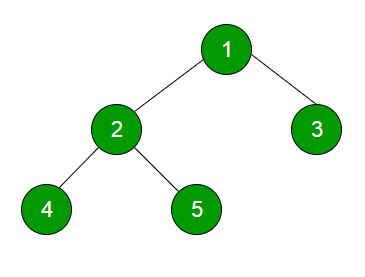 1, 2, 3, 4, 5
# Iterative with queue - time O(n), space O(n)
class Node:
    # create a new node
    def __init__(self, key):
        self.val = key
        self.left = None
        self.right = None

# print height
def LevelOrder(root):

    # base case
    if root is None:
        return

    queue = []
    queue.append(root)

    while(len(queue) > 0):

        node = queue.pop(0)                 # print and remove front of queue
        print(node.val, end=' ')

        if node.left is not None:
            queue.append(node.left)

        if node.right is not None:
            queue.append(node.right)
# Recursive - time O(n^2), space O(n)
class Node:

    # create a new node
    def __init__(self, val):
        self.val = val
        self.left = None
        self.right = None


# print level order traversal
def LevelOrder_rec(root):
    h = height(root)
    for i in range(1, h+1):
        printGivenLevel(root, i)


# print nodes at a given level
def printGivenLevel(root , level):
    if root is None:
        return
    if level == 1:
        print(root.val, end=" ")
    elif level > 1 :
        printGivenLevel(root.left , level-1)                         # if saving in a list: res += printGivenLevel()
        printGivenLevel(root.right , level-1)


# compute height - number of nodes from root to farthest leaf node
def height(node):
    if node is None:
        return 0
    else :
        # Compute the height of each subtree
        lheight = height(node.left)
        rheight = height(node.right)

        #Use the larger one
        if lheight > rheight :
            return lheight+1
        else:
            return rheight+1
root = Node(1)
root.left = Node(2)
root.right = Node(3)
root.left.left = Node(4)
root.left.right = Node(5)

print("Recursive level order traversal:")
LevelOrder_rec(root)

print("\nQueue-based level order traversal:")
LevelOrder(root)
Recursive level order traversal:
1 2 3 4 5
Queue-based level order traversal:
1 2 3 4 5
# StackOverflow
class Solution:
    def inorderTraversal(self, root):
        return (self.inorderTraversal(root.left) + [root.val] + self.inorderTraversal(root.right)) if root else []
TREE SOLUTIONS
# A full BT = BT where every node has either 0 or 2 children. Examples:
'''
        1
      /   \
    2       3
  /  \     /  \
 4    5   6    7


       1
     /   \
   2      3
        /   \
       4     5
           /   \
          6    7


          1
        /   \
      2       3
    /  \     /  \
   4    5   6    7
 /  \
8    9
'''
pass
Another way to build a BT
class Node:

    def __init__(self, data, left=None, right=None):
        self.val = data
        self.left = left
        self.right = right

# Left Root Right
def inorder(root):

    if root:
        inorder(root.left)
        print(root.val, end=' '),
        inorder(root.right)

root = Node(1,
            right = Node(3),
            left  = Node(2,
                         left = Node(4),
                         right = Node(5)
            )
       )
Inorder(root)
4 2 5 1 3
Check if tree is BST
"""
Given a binary tree, determine if it is a valid binary search tree (BST).

Assume a BST is defined as follows:

The left subtree of a node contains only nodes
with keys less than the node's key.
The right subtree of a node contains only nodes
with keys greater than the node's key.
Both the left and right subtrees must also be binary search trees.
Example 1:
    2
   / \
  1   3
Binary tree [2,1,3], return true.
Example 2:
    1
   / \
  2   3
Binary tree [1,2,3], return false.
# Udemy
# If a tree is BST => inorder traversal outputs a sorted list
tree_vals = []

def inorder( tree ):
    if tree != None:
        inorder(tree.getLeftChild())
        tree_vals.append(tree.getRootVal())
        inorder(tree.getRightChild())

def sort_check( tree_vals ):
    return tree_vals == sorted(tree_vals)                # just iterate list for O(n) solution

inorder(tree)
sort_check(tree_vals)
# Udemy
# Another classic solution: keep track of min and max values a node can take - at each node we check if its value
# is between min and max values it’s allowed to take. Root = any value between neg infinity and pos infinity.
# Left child should be smaller than or equal than root, right child should be larger than or equal to root.
# During recursion, send current value as new max to left child and send min without changing.
# Send current value as new min to right child and send max without changing

class Node:
    def __init__(self, k, val):
        self.key = k
        self.value = val
        self.left = None
        self.right = None

def tree_max(node):
    if not node:
        return float("-inf")
    maxleft  = tree_max(node.left)
    maxright = tree_max(node.right)
    return max(node.key, maxleft, maxright)

def tree_min(node):
    if not node:
        return float("inf")
    minleft  = tree_min(node.left)
    minright = tree_min(node.right)
    return min(node.key, minleft, minright)

def verify(node):
    if not node:
        return True
    if (tree_max(node.left) <= node.key <= tree_min(node.right) and
        verify(node.left) and verify(node.right)):
        return True
    else:
        return False
root= Node(10, "Hello")
root.left = Node(5, "Five")
root.right= Node(30, "Thirty")

print(verify(root)) # prints True, since this tree is valid

root = Node(10, "Ten")
root.right = Node(20, "Twenty")
root.left = Node(5, "Five")
root.left.right = Node(15, "Fifteen")

print(verify(root)) # prints False, since 15 is to the left of 10
True
False
Count BST nodes that lie in a given range
#Time c. O(h + k) where h = tree hight and k = num nodes in range
class newNode:

    # Constructor for a new node
    def __init__(self, data):
        self.data = data
        self.left = None
        self.right = None

# Returns count of nodes in BST in range [low, high]
def getCount(root, low, high):

    # Base case
    if root == None:
        return 0

    # Special case
    if root.data == high and root.data == low:
        return 1

    # If current node in range => include it in count and recur for left & right children
    if root.data <= high and root.data >= low:
        return (1 + getCount(root.left, low, high) + getCount(root.right, low, high))

    # If current node < low, recur for right child
    elif root.data < low:
        return getCount(root.right, low, high)

    # Else recur for left child
    else:
        return getCount(root.left, low, high)


# Let us construct the BST shown in
# the above figure
root = newNode(10)
root.left = newNode(5)
root.right = newNode(50)
root.left.left = newNode(1)
root.right.left = newNode(40)
root.right.right = newNode(100)

# Let us constructed BST shown in above example
#         10
#       /   \
#     5     50
#   /       / \
#  1       40 100

l = 5
h = 45
print("Count of nodes between [", l, ", ", h,"] is ", getCount(root, l, h))
Count of nodes between [ 5 , 45 ] is 3
Find a BST node whose value is closest to a target floating point number
# Note:
# Given target value is a floating point => you are guaranteed to have only one unique closest value in BST

# Definition for a binary tree node.
# class TreeNode(object):
#     def __init__(self, x):
#         self.val = x
#         self.left = None
#         self.right = None

def closest_value(root, target):

    a = root.val
    child = root.left if target < a else root.right
    if not child:
        return a
    b = closest_value(child, target)

    return min(target-a, target-b)
"""
Write f(x) count_left_node() to return num of left children in tree.
For example: four left children here (6, 3, 7, and 10):

                    9
                 /      \
               6         12
              / \       /   \
            3     8   10      15
                 /              \
                7                18

    count_left_node = 4

"""
from bst import Node
from bst import bst

def count_left_node(root):

    if root is None:
        return 0
    elif root.left is None:
        return count_left_node( root.right )
    else:
        return 1 + count_left_node(root.left) + count_left_node(root.right)
"""
Implement a trie with insert, search, and startsWith methods.

Note:
You may assume that all inputs consist of lowercase letters a-z.
"""
from collections import defaultdict


class TrieNode:
    def __init__(self):
        self.children = defaultdict(TrieNode)
        self.is_word = False


class Trie:
    def __init__(self):
        self.root = TrieNode()

    def insert(self, word):
        current = self.root
        for letter in word:
            current = current.children[letter]
        current.is_word = True

    def search(self, word):
        current = self.root
        for letter in word:
            current = current.children.get(letter)
            if current is None:
                return False
        return current.is_word

    def starts_with(self, prefix):
        current = self.root
        for letter in prefix:
            current = current.children.get(letter)
            if current is None:
                return False
        return True
Trim BST (Udemy)
Given root of BST and 2 numbers min and max, trim BST by removing all nodes w/values not between min and max (inclusive). The resulting tree should still be a valid BST. If this is input:
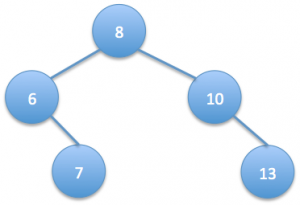
and we’re given min value as 5 and max value as 13, this should be the output:
Solution
We can do this by performing a post-order traversal of the tree. We first process the left children, then right children, and finally the node itself. So we form the new tree bottom up, starting from the leaves towards the root. As a result while processing the node itself, both its left and right subtrees are valid trimmed binary search trees (may be NULL as well).
At each node we’ll return a reference based on its value, which will then be assigned to its parent’s left or right child pointer, depending on whether the current node is left or right child of the parent. If current node’s value is between min and max (min<=node<=max) then there’s no action needed, so we return the reference to the node itself. If current node’s value is less than min, then we return the reference to its right subtree, and discard the left subtree. Because if a node’s value is less than min, then its left children are definitely less than min since this is a binary search tree. But its right children may or may not be less than min we can’t be sure, so we return the reference to it. Since we’re performing bottom-up post-order traversal, its right subtree is already a trimmed valid binary search tree (possibly NULL), and left subtree is definitely NULL because those nodes were surely less than min and they were eliminated during the post-order traversal. Remember that in post-order traversal we first process all the children of a node, and then finally the node itself.
Similar situation occurs when node’s value is greater than max, we now return the reference to its left subtree. Because if a node’s value is greater than max, then its right children are definitely greater than max. But its left children may or may not be greater than max. So we discard the right subtree and return the reference to the already valid left subtree. The code is easier to understand:
def trimBST(tree, minVal, maxVal):

    if not tree:
        return

    tree.left=trimBST(tree.left, minVal, maxVal)
    tree.right=trimBST(tree.right, minVal, maxVal)

    if minVal<=tree.val<=maxVal:
        return tree

    if tree.val < minVal:
        return tree.right

    if tree.val > maxVal:
        return tree.left
The complexity of this algorithm is O(N), where N is the number of nodes in the tree. Because we basically perform a post-order traversal of the tree, visiting each and every node one. This is optimal because we should visit every node at least once. This is a very elegant question that demonstrates the effectiveness of recursion in trees.
Check if two BTs are equal (recursive)
"""
Two binary trees are considered equal if they are
structurally identical and the nodes have the same value.
"""


def is_same_tree(p, q):
    if not p and not q:
        return True
    if p and q and p.val == q.val:
        return is_same_tree(p.left, q.left) and is_same_tree(p.right, q.right)
    return False

# Time Complexity O(min(N,M))
# where N and M are the number of nodes for the trees.

# Space Complexity O(min(height1, height2))
# levels of recursion is the mininum height between the two trees.
Invert a binary tree
def reverse(root):

    if not root:
        return
    root.left, root.right = root.right, root.left

    if root.left:
        reverse(root.left)
    if root.right:
        reverse(root.right)
Find deepest left node
# Given a binary tree, find the deepest node
# that is the left child of its parent node.

# Example:

     # 1
   # /   \
  # 2     3
 # / \     \
# 4   5     6
           # \
            # 7
# should return 4.


class Node:
    def __init__(self, val = None):
        self.val = val
        self.left = None
        self.right = None


class DeepestLeft:
    def __init__(self):
        self.depth = 0
        self.Node = None

def find_deepest_left(root, is_left, depth, res):
    if not root:
        return
    if is_left and depth > res.depth:
        res.depth = depth
        res.Node = root
    find_deepest_left(root.left, True, depth + 1, res)
    find_deepest_left(root.right, False, depth + 1, res)

root = Node(1)
root.left = Node(2)
root.right = Node(3)
root.left.left = Node(4)
root.left.right = Node(5)
root.right.right = Node(6)
root.right.right.right = Node(7)

res = DeepestLeft()
find_deepest_left(root, True, 1, res)
if res.Node:
    print(res.Node.val)
4
Min / Max height
"""
Maximum depth = # nodes along the longest path from root to farthest leaf node.
"""


class Node():
    def __init__(self, val = 0):
        self.val = val
        self.left = None
        self.right = None


def max_height(root):

    if not root:
        return 0
    return max(max_height(root.left), max_height(root.right)) + 1


def min_height(root):

    if not root:
        return 0

    if not root.left or not root.right:
        return max(min_height(root.left), min_height(root.right))+1

    return min(min_height(root.left), min_height(root.right)) + 1


def print_tree(root):
    if root:
        print(root.val, end=' ')
        print_tree(root.left)
        print_tree(root.right)
tree = Node(10)
tree.left = Node(12)
tree.right = Node(15)
tree.left.left  = Node(25)
tree.left.left.right  = Node(100)
tree.left.right = Node(30)
tree.right.left = Node(36)

print_tree(tree)
print()

maxHeight = max_height(tree)
print("Max height:", maxHeight)

minHeight = min_depth(tree)
print("Min height:", minHeight)
10 12 25 100 30 15 36
Max height: 4
Min height: 3
Check if BT is balanced
def is_balanced(root):
    """
    O(N) solution
    """
    return -1 != get_depth(root)

def get_depth(root):
    """
    return 0 if unbalanced else depth + 1
    """
    if not root:
        return 0
    left  = get_depth(root.left)
    right = get_depth(root.right)
    if abs(left-right) > 1 or left == -1 or right == -1:
        return -1
    return 1 + max(left, right)

################################

def is_balanced(root):
    """
    O(N^2) solution
    """
    left = max_height(root.left)
    right = max_height(root.right)
    return abs(left-right) <= 1 and is_balanced(root.left) and is_balanced(root.right)

def max_height(root):
    if not root:
        return 0
    return max(max_height(root.left), max_height(root.right)) + 1
Lowest common ancestor - any binary tree (accepted on LeetCode)
"""
Given a binary tree, find the lowest common ancestor
(LCA) of two given nodes in the tree.

According to the definition of LCA on Wikipedia:
    “The lowest common ancestor is defined between two nodes
    v and w as the lowest node in T that has both v and w as
    descendants
    (where we allow a node to be a descendant of itself).”

        _______3______
       /              \
    ___5__          ___1__
   /      \        /      \
   6      _2       0       8
         /  \
         7   4
For example, the lowest common ancestor (LCA) of nodes 5 and 1 is 3.
Another example is LCA of nodes 5 and 4 is 5,
since a node can be a descendant of itself according to the LCA definition.
"""


def lca(root, p, q):
    """
    :type root: TreeNode
    :type p: TreeNode
    :type q: TreeNode
    :rtype: TreeNode
    """
    if not root or root is p or root is q:
        return root
    left = lca(root.left, p, q)
    right = lca(root.right, p, q)
    if left and right:
        return root
    return left if left else right
Lowest common ancestor - binary search tree only (Geeks for geeks)
# Time c. O(h), space c. O(1)
class Node:

    def __init__(self, data):
        self.data = data
        self.left = None
        self.right = None

# Assuming that both n1 and n2 are present in BST
def lca(root, n1, n2):

    if root is None:                                                            # Base Case
        return None

    # If both n1 & n2 < root, then LCA lies in left
    if(root.data > n1 and root.data > n2):
        return lca(root.left, n1, n2)

    # If both n1 & n2 > root, then LCA lies in right
    if(root.data < n1 and root.data < n2):
        return lca(root.right, n1, n2)

    return root


root = Node(20)
root.left = Node(8)
root.right = Node(22)
root.left.left = Node(4)
root.left.right = Node(12)
root.left.right.left = Node(10)
root.left.right.right = Node(14)

n1 = 10 ; n2 = 14
t = lca(root, n1, n2)
print('LCA of %d and %d is %d' %(n1, n2, t.data))

n1 = 14 ; n2 = 8
t = lca(root, n1, n2)
print('LCA of %d and %d is %d' %(n1, n2 , t.data))

n1 = 10 ; n2 = 22
t = lca(root, n1, n2)
print('LCA of %d and %d is %d' %(n1, n2, t.data))
LCA of 10 and 14 is 12
LCA of 14 and 8 is 8
LCA of 10 and 22 is 20
Maximum path sum
def max_path_sum(root):
    max_sum = float('-inf')
    def gain(root):
        nonlocal max_sum
        if not root: return 0
        # only pos values
        left  = max(gain(root.left), 0)
        right = max(gain(root.right),0)
        # update global max_sum
        new_path = root.val+left+right
        max_sum = max(max_sum, new_path)
        # return max gain if continue same path up
        return root.val + max(left, right)
    gain(root)
    return max_sum
class Node:
    def __init__(self, val=None):
        self.val = val
        self.left = None
        self.right = None

root = Node(20)
root.left = Node(8)
root.right = Node(22)
root.left.left = Node(4)
root.left.right = Node(12)
root.left.right.left = Node(10)
root.left.right.right = Node(15)

max_path_sum(root)
77
Check if BT has a path sum
"""
Given a binary tree and a sum, determine if the tree has a root-to-leaf
path such that adding up all the values along the path equals the given sum.

For example:
Given the below binary tree and sum = 22,
              5
             / \
            4   8
           /   / \
          11  13  4
         /  \      \
        7    2      1
return true, as there exist a root-to-leaf path 5->4->11->2 which sum is 22.
"""
class Node:
    def __init__(self, val = 0):
        self.val = val
        self.left = None
        self.right = None


def has_path_sum(root, sum):
    """
    :type root: TreeNode
    :type sum: int
    :rtype: bool
    """
    if not root:
        return False
    if not root.left and not root.right and root.val == sum:
        return True
    sum -= root.val
    return has_path_sum(root.left, sum) or has_path_sum(root.right, sum)


# DFS with stack
def has_path_sum2(root, sum):
    if not root:
        return False
    stack = [(root, root.val)]
    while stack:
        node, val = stack.pop()
        if not node.left and not node.right:
            if val == sum:
                return True
        if node.left:
            stack.append((node.left, val+node.left.val))
        if node.right:
            stack.append((node.right, val+node.right.val))
    return False


# BFS with queue
def has_path_sum3(root, sum):
    if not root:
        return False
    queue = [(root, sum-root.val)]
    while queue:
        node, val = queue.pop(0)  # popleft
        if not node.left and not node.right:
            if val == 0:
                return True
        if node.left:
            queue.append((node.left, val-node.left.val))
        if node.right:
            queue.append((node.right, val-node.right.val))
    return False

tree = Node(10)
tree.left = Node(12)
tree.right = Node(15)
tree.left.left  = Node(25)
tree.left.left.right  = Node(100)
tree.left.right = Node(30)
tree.right.left = Node(36)

print_tree(tree)
print()

# see why it is not working as expected
for i in range(500):
    if has_path_sum(tree, i):
        print(i)
10 12 25 100 30 15 36
52
61
147
Sorted array to BST
"""
Given an array where elements are sorted in ascending order,
convert it to a height balanced BST.
"""


class TreeNode(object):
    def __init__(self, x):
        self.val = x
        self.left = None
        self.right = None


def array_to_bst(nums):
    if not nums:
        return None
    mid = len(nums)//2
    node = TreeNode(nums[mid])
    node.left = array_to_bst(nums[:mid])
    node.right = array_to_bst(nums[mid+1:])
    return node
Trees - Top 10 Algorithms in Interview Questions (Geeksforgeeks.com)
Distance between two nodes of a Binary Tree
Using lowest common ancestor (LCA):
Dist(n1, n2) = Dist(root, n1) + Dist(root, n2) - 2*Dist(root, LCA) 'n1' and 'n2' are the two given nodes (their values)
Time c. O(n)?
# binary tree node
class Node:

    def __init__(self, data):
        self.data = data
        self.left = self.right = None


# find LCA
def LCA(root, n1, n2):

    # Base case
    if root is None:
        return None

    if root.data == n1 or root.data == n2:
        return root

    # Look for keys in left and right subtrees
    left = LCA(root.left, n1, n2)
    right = LCA(root.right, n1, n2)

    if left is not None and right is not None:
        return root

    if left:
        return left
    else:
        return right


# find distance of any node from root
def findLevel(root, data, d, level):

    if root is None:                                                           # base case
        return

    if root.data == data:                                                      # node found
        d.append(level)
        return

    findLevel(root.left, data, d, level + 1)
    findLevel(root.right, data, d, level + 1)


def findDistance(root, n1, n2):

    lca = LCA(root, n1, n2)
    d1 = []                                                                    # distance(n1, lca)
    d2 = []                                                                    # distance(n2, lca)


    if lca:                                                                    # if lca exist

        findLevel(lca, n1, d1, 0)
        findLevel(lca, n2, d2, 0)
        return d1[0] + d2[0]

    else:
        return -1


root = Node(1)
root.left = Node(2)
root.right = Node(3)
root.left.left = Node(4)
root.left.right = Node(5)
root.right.left = Node(6)
root.right.right = Node(7)
root.right.left.right = Node(8)

print("Dist(4,5) = ", findDistance(root, 4, 5))
print("Dist(4,6) = ", findDistance(root, 4, 6))
print("Dist(3,4) = ", findDistance(root, 3, 4))
print("Dist(2,4) = ", findDistance(root, 2, 4))
print("Dist(8,5) = ", findDistance(root, 8, 5))
Dist(4,5) =  2
Dist(4,6) =  4
Dist(3,4) =  3
Dist(2,4) =  1
Dist(8,5) =  5
Maximum Path Sum in a Binary Tree
Four ways that the max path goes through each node: 1. Node only 2. Max path through Left Child + Node 3. Max path through Right Child + Node 4. Max path through Left Child + Node + Max path through Right Child
Keep track of the four paths and pick the max one in the end. Important: root of every subtree need to return max path sum such that at most one child of root is involved - needed for parent function call. In below code, this sum is stored in 'max_single' and returned by the recursive function
# A Binary Tree Node
class Node:

    # Contructor to create a new node
    def __init__(self, data):
        self.data = data
        self.left = None
        self.right = None


# Return maximum path sum in 'res' + return max path sum going through root
def findMaxUtil(root):

    # base case
    if root is None:
        return 0

    l = findMaxUtil(root.left)
    r = findMaxUtil(root.right)

    max_single = max(max(l, r) + root.data, root.data)

    max_top = max(max_single, l + r + root.data)

    # Static variable to store the maximum result
    findMaxUtil.res = max(findMaxUtil.res, max_top)

    return max_single


# Return max path sum in tree with given root
def findMaxSum(root):

    # Initialize result
    findMaxUtil.res = float("-inf")

    # Compute and return result
    findMaxUtil(root)
    return findMaxUtil.res

root = Node(10)
root.left = Node(2)
root.right   = Node(10);
root.left.left  = Node(20);
root.left.right = Node(1);
root.right.right = Node(-25);
root.right.right.left   = Node(3);
root.right.right.right  = Node(4);
print("Max path sum is " ,findMaxSum(root))
Max path sum is 42
Check if a binary tree is full
A full binary tree (BT) - all nodes have either zero or two child nodes OR no node has one child node:
1) If a BT node is NULL => full BT
2) If a BT node has empty left and right sub-trees => full BT (a leaf node)
3) If a BT node has left and right sub-trees => it's part of a full BT, recursively check its left and right sub-trees
4) Any other case => not a full BT
# BT node
class Node:

    def __init__(self , key):
        self.key = key
        self.left = None
        self.right = None


def isFullTree(root):

    # If empty tree
    if root is None:
        return True

    # If a leaf node
    if root.left is None and root.right is None:
        return True

    # If both left & right subtrees != None and are full
    if root.left is not None and root.right is not None:
        return (isFullTree(root.left) and isFullTree(root.right))

    # If we reach here - none of the above conditions held
    return False

# Driver Program
root = Node(10);
root.left = Node(20);
root.right = Node(30);

root.left.right = Node(40);
root.left.left = Node(50);
root.right.left = Node(60);
root.right.right = Node(70);

root.left.left.left = Node(80);
root.left.left.right = Node(90);
root.left.right.left = Node(80);
root.left.right.right = Node(90);
root.right.left.left = Node(80);
root.right.left.right = Node(90);
root.right.right.left = Node(80);
root.right.right.right = Node(90);

if isFullTree(root):
    print('BT is full')
else:
    print('BT is not full')
BT is full
Check if a binary tree is subtree of another binary tree
Traverse the tree T in preorder fashion. For every visited node in the traversal, see if the subtree rooted with this node is identical to S.
Time c. O(mn) in worst case where m & n # nodes in the given two trees. O(n) is possible, but not clear on Geeksforgeeks (and doesn't have a Python version)
# BT node
class Node:
    def __init__(self, data):
        self.data = data
        self.left = None
        self.right = None

# check if two trees are identical
def areIdentical(root1, root2):

    if root1 is None and root2 is None:                                             # base case
        return True
    if root1 is None or root2 is None:
        return False

    # check both roots are the same and left & right subtrees are the same
    return (root1.data == root2.data and
            areIdentical(root1.left , root2.left) and
            areIdentical(root1.right, root2.right)
            )

# check if subtree
def isSubtree(T, S):

    if S is None:                                                                    # base case
        return True

    if T is None:
        return False

    if (areIdentical(T, S)):
        return True

    # if none of the above try left and right subtrees one by one
    return isSubtree(T.left, S) or isSubtree(T.right, S)


""" TREE 1
     Construct the following tree
              26
            /   \
          10     3
        /    \     \
       4      6     3
       \
        30
    """

T = Node(26)
T.right = Node(3)
T.right.right  = Node(3)
T.left = Node(10)
T.left.left = Node(4)
T.left.left.right = Node(30)
T.left.right = Node(6)

""" TREE 2
     Construct the following tree
          10
        /    \
       4      6
        \
         30
    """
S = Node(10)
S.right = Node(6)
S.left = Node(4)
S.left.right = Node(30)

if isSubtree(T, S):
    print('Tree 2 is subtree of Tree 1')
else:
    print('Tree 2 is not a subtree of Tree 1')
Tree 2 is subtree of Tree 1
Reverse alternate levels of a perfect binary tree
A simple solution is to do following steps:
1) Access nodes level by level.
2) If current level is odd, then store nodes of this level in an array.
3) Reverse the array and store elements back in tree.
"""
Given tree:
               a
            /     \
           b       c
         /  \     /  \
        d    e    f    g
       / \  / \  / \  / \
       h  i j  k l  m  n  o

Modified tree:
               a
            /     \
           c       b
         /  \     /  \
        d    e    f    g
       / \  / \  / \  / \
      o  n m  l k  j  i  h
"""

class Node:

    def __init__(self, key):
        self.key = key
        self.left = None
        self.right = None


def preorder(root1, root2, lvl):

    if (root1 == None or root2 == None):                                  # base case
        return

    if (lvl % 2 == 0):                                                    # swap subtrees if level is even
        t = root1.key
        root1.key = root2.key
        root2.key = t

    preorder(root1.left, root2.right, lvl + 1)                            # recur for left and right subtrees
    preorder(root1.right, root2.left, lvl + 1)


def reverseAlternate(root):
    preorder(root.left, root.right, 0)


# inorder traversal (print initial trees)
def printInorder(root):

    if (root == None):
        return

    printInorder(root.left)
    print( root.key, end = " ")
    printInorder(root.right)


root = Node('a')
root.left = Node('b')
root.right = Node('c')
root.left.left = Node('d')
root.left.right = Node('e')
root.right.left = Node('f')
root.right.right = Node('g')
root.left.left.left = Node('h')
root.left.left.right = Node('i')
root.left.right.left = Node('j')
root.left.right.right = Node('k')
root.right.left.left = Node('l')
root.right.left.right = Node('m')
root.right.right.left = Node('n')
root.right.right.right = Node('o')

print( "Inorder traversal of initial tree")
printInorder(root)

reverseAlternate(root)

print("\nInorder traversal of modified tree")
printInorder(root)
Inorder traversal of initial tree
h d i b j e k a l f m c n g o
Inorder traversal of modified tree
o d n c m e l a k f j b i g h
Print Nodes of Binary Tree in Top View (aka External Nodes)
Top view - nodes visible when the tree is viewed from the top (printed in any order). Expected time complexity is O(n). Not too clear what a top view is - why 6 in the second example below is printed last? Because of in any order?
'''
       1
    /     \
   2       3
  /  \    / \
 4    5  6   7
Top view of the above binary tree is
4 2 1 3 7

        1
      /   \
    2       3
      \
        4
          \
            5
             \
               6
Top view of the above binary tree is
2 1 3 6
'''

class Node:
    def __init__(self, key):
        self.data = key
        self.left = None
        self.right = None

# f(x) to fill the map
def fillMap(root, d, l, m):
    if(root == None):
        return

    if d not in m:
        m[d] = [root.data,l]
    elif(m[d][1] > l):
        m[d] = [root.data,l]
    fillMap(root.left, d - 1, l + 1, m)
    fillMap(root.right, d + 1, l + 1, m)

# f(x) to print top view of BT
def topView(root):

    # map to store the pair of node value and its level
    # with respect to the vertical distance from root.
    m = {}

    fillMap(root, 0, 0, m)
    for it in sorted (m.keys()):
        print(m[it][0], end = " ")


root = Node(1)
root.left = Node(2)
root.right = Node(3)
root.left.right = Node(4)
root.left.right.right = Node(5)
root.left.right.right.right = Node(6)
print('Following are nodes in top view of Binary Tree')
topView(root)
Following are nodes in top view of Binary Tree
2 1 3 6