MLE vs. Bayesian Estimation
Parameter estimation aims to infer the model and population distribution that most likely generated the observed data. Two major approaches:
Maximum Likelihood Estimation (MLE) – Frequentist view: probability = long-run relative frequency.
Bayesian Estimation (BE) – Bayesian view: probability = degree of belief, updated with data.
Maximum Likelihood Estimation (MLE)
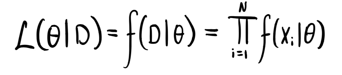
Based on the likelihood function: the probability of observing the data given specific parameters.
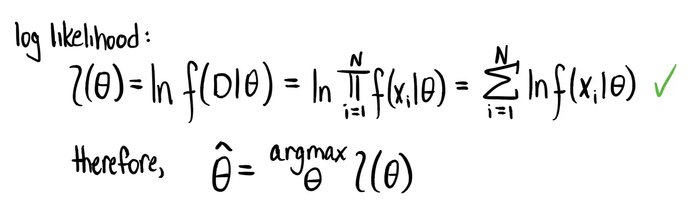
The MLE estimate theta_hat is the parameter set that maximizes this likelihood.
In practice, the log-likelihood is used for numerical stability (sum of logs instead of product of probabilities).
Intuition: finds the parameter values that make the observed data most probable under the model.
On the left - Likelihood function = product of probabilities - chance that each possible parameter value produced the data we observed (assumption – data samples are independent).
On the right - Log likelihood = avoids multiplying many numbers and getting very low values (and log of product = sum of logs):
 |
 |
Bayesian Estimation (BE)
Incorporates prior knowledge (prior distribution) about parameters before observing data.
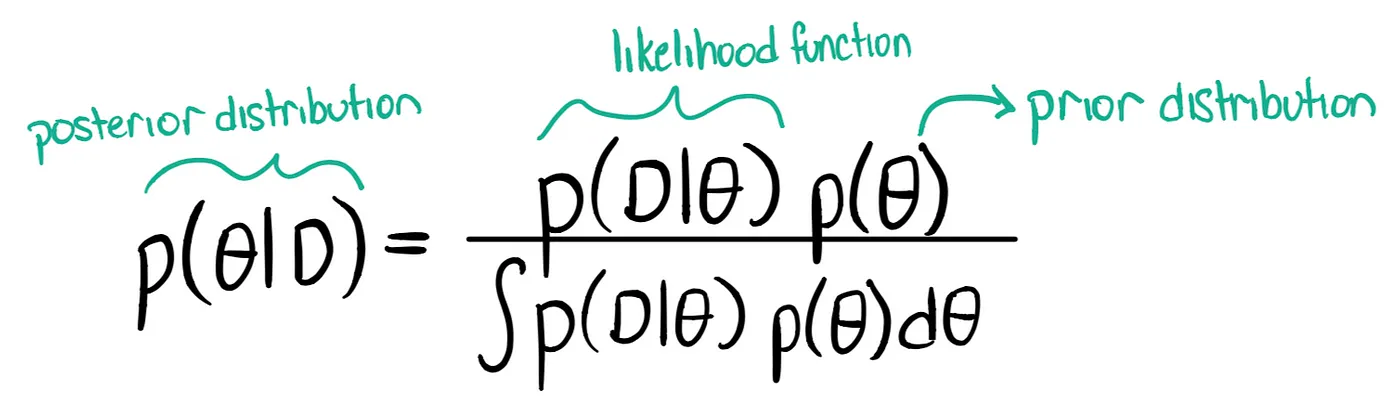 Updates beliefs using Bayes’ theorem:
Result is the posterior distribution, representing our updated belief about parameter values after seeing data.
More computationally intensive, since normalization often requires integration.
Comparison
MLE:
Pros – simple, efficient with large data.
Cons – biased when data is scarce, ignores prior knowledge.
Bayesian Estimation:
Pros – leverages prior knowledge, more robust with small datasets.
Cons – requires well-defined, reliable priors (or the model is biased); computationally more complex (use them if not constrained by resources).
Rule of thumb:
Use MLE when data is abundant and priors are unreliable.
Use Bayesian estimation when data is limited or reliable priors exist, and resources allow.