DL Basics
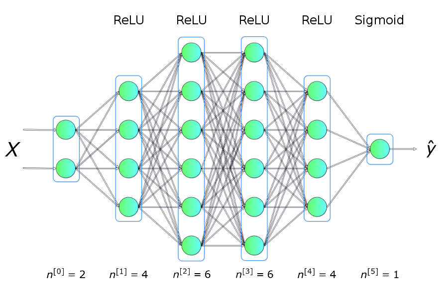
DL = Subset of ML based on neural networks. Each layer transforms its inputs into progressively higher-level features. Deep networks = neural networks with multiple hidden layers.
Neural networks are “universal approximators” - with enough layers and neurons, they can represent almost any function.
Popular Architectures:
Linear Classifier – simplest form, predicts based on weighted input features (stack of linear layers + one single linear transformation).
Don’t confuse linear classifier w/perceptron which is a basic unit of a neural network (neuron) - a single linear model + nonlinear activation. Perceptron becomes linear if you remove the nonlinear activation.
DNN (Deep Neural Networks) – multiple hidden layers with nonlinear activations.
CNN (Convolutional Neural Networks) – convolution + pooling layers, widely used for image tasks.
RNN (Recurrent Neural Networks, LSTMs) – handle sequential data by maintaining memory.
GANs (Generative Adversarial Networks) – generate synthetic examples via generator–discriminator setup.
Transfer Learning – reuse pretrained models for new tasks.
Wide & Deep – hybrid of linear + deep models for structured data.
Core Building Blocks
Neuron: Node in a neural network, takes inputs, applies an activation function (nonlinear transformation), and outputs a value.
Neural Network: Composition of neurons and activation functions that enable nonlinear predictions.
Weights / Biases: Parameters multiplied with inputs to produce outputs. Weights control feature contribution; biases shift the output.
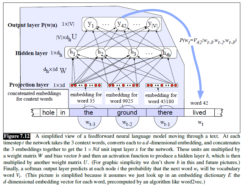
Embeddings: Mapping from discrete objects (like words) to vectors of real numbers, useful for classification tasks.
Activation Functions
Activation Functions: Mathematical functions that introduce non-linearity into a network (e.g., ReLU, tanh).
Sigmoid Function: Maps values to the range (0, 1), often used for predicting probabilities.
Optimization & Training
Gradient Descent / Backpropagation: Core optimization methods for adjusting weights based on error gradients.
Optimizer: Algorithms that update weights and biases to minimize loss (e.g., SGD, Adam).
Learning Rate: Controls step size in optimization; high values train faster but risk divergence, low values converge more slowly.
Converge: When an algorithm eventually reaches an optimal (or near-optimal) solution.
Training Challenges
Numerical Instability: Issues from floating point limits with very large/small values.
Overfitting Controls:
Dropout: Regularization by randomly removing units in a network layer during training.
Early Stopping: Regularization by halting training before overfitting occurs.
Neural Network Layers & Operations
Convolutional Layer: Applies convolution operations across input data (commonly in CNNs) to capture spatial features.
Pooling: reducing matrix from an earlier convolutional layer to a smaller matrix – taking the max or average value across the pooled area. Pooling mainly helps in extracting sharp, low-level features like edges, points (max pool) and smooth features (average pool). It is also done to reduce variance and computations.
CNN Essentials
CNNs use convolutions (with stride, padding, and multiple filters), pooling, and fully connected layers to progressively learn and combine features, making them the dominant method for visual recognition tasks.
Introduction
CNNs excel at image tasks by preserving spatial layout and automatically learning features (edges, textures, shapes).
Convolutional layers replace manual feature engineering, enabling accuracy and scalability.
Architecture
CNNs mimic the human visual system with key layers: convolutional layers, activation functions, pooling layers, and fully connected layers.
Key Components
Convolutional Layers: applies small learnable filters (kernels) that slide across the input to detect local patterns like edges or textures. Each filter produces a feature map showing where that pattern occurs. This operation uses local connectivity and weight sharing, enabling the network to efficiently learn spatial features and build hierarchical representations of images.
Stride: Step size for moving filters; small strides preserve detail, large strides reduce resolution and computation.
Padding: Zero-padding around inputs to control feature map size; “valid” = no padding, “same” = preserve dimensions.
Multiple Filters & Depth: Each filter learns distinct features; stacking feature maps builds hierarchical representations.
Weight Sharing: Reuses the same filter across input → reduces parameters, improves efficiency, enables translation invariance.
Feature Maps: Outputs of convolution operations showing where features are detected.
Pooling Layers
Reduce feature map dimensions, retaining essential information while lowering computation.
Types: Max pooling (captures strongest features), average pooling (generalized features), global pooling (single value per map).
Fully Connected Layers
Feed-forward network layers (CNN): input layer, hidden layers w/dropout, output layer
Flatten feature maps into vectors for global reasoning.
Learn high-level patterns and perform classification (SoftMax - multiclass).