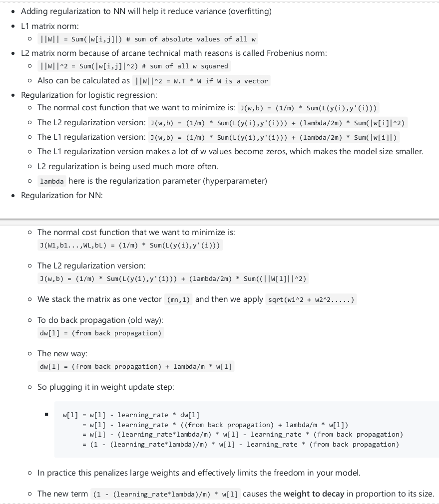
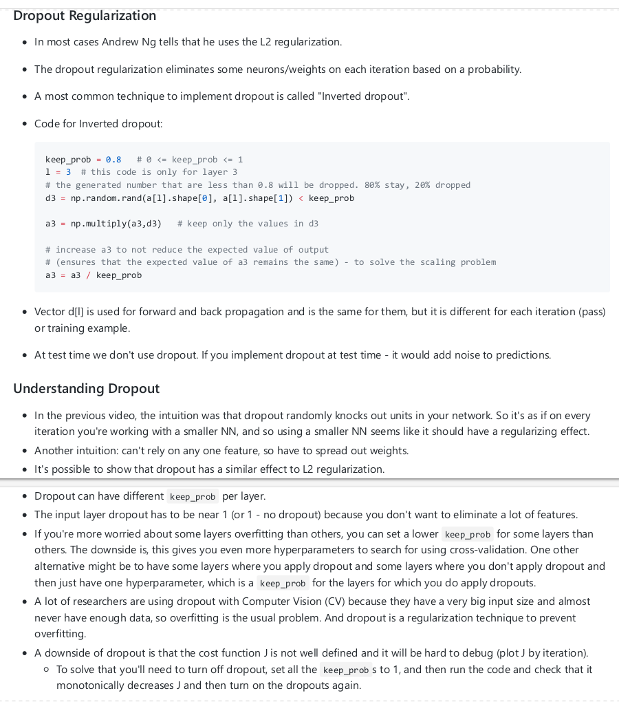
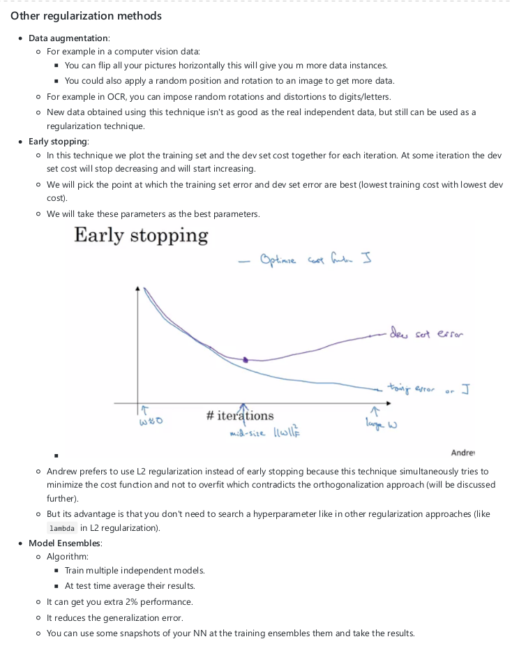
DIMENSIONALITY REDUCTION
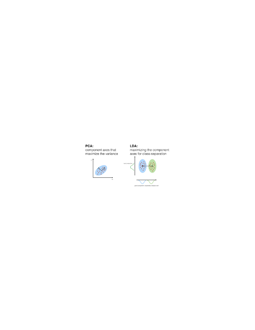
PCA UNSUPERVISED statistical technique to reduce the dimensionality of dataset while retaining most of its important information.
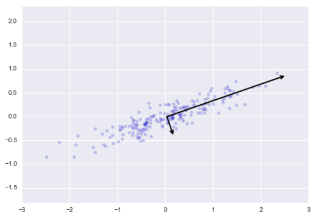
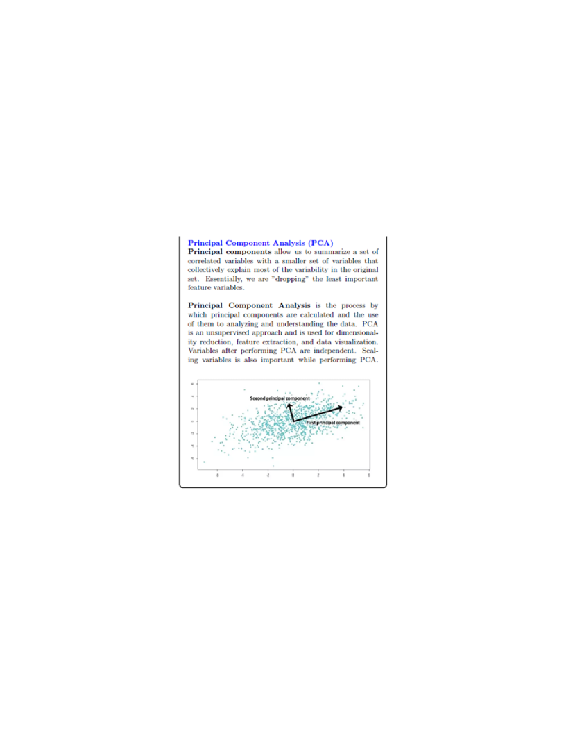
It does this by finding new axes — called principal components — that are linear combinations of the original features and capture the directions of maximum variance in the data. The first principal component explains the greatest amount of variation, the second explains the next most (while being orthogonal to the first), and so on. This simplifies complex datasets, reduces noise, and improves visualization or computational efficiency in ML. PCA = zeroing out one or more of smallest principal components, resulting in a lower-dimensional projection of the data that preserves the maximal data variance. Incorporate (if needed):
|
LDA SUPERVISED dimensionality reduction as a linear transformation, computes the directions (“linear discriminants”) that will represent the axes that maximize the separation between multiple classes. LDA not always superior to PCA for a multi-class classification, e.g. image recognition if the number of samples per class is relatively small - PCA outperforms. In practice, it is not uncommon to use both LDA and PCA in combination: e.g. PCA for dimensionality reduction followed by LDA
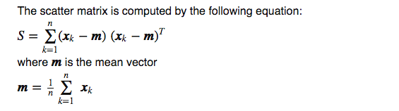
Scatter matrix - estimation of covariance matrix (if the latter is costly). For k vars, s. m. has k rows and k cols
|
|
|---|---|---|
 |

PCA Summary
Standardize range of continuous vars (subtracting mean, dividing by standard deviation).
Compute the covariance matrix to identify correlations among vars.
Compute the eigenvectors ( directions in which data is dispersed) and eigenvalues (magnitudes of eigenvectors) of the covariance matrix = principal components.
Create a feature vector to decide which PC to keep (which eigenvectors are relatively important).
Recast data along the principal components axes.
When use PCA: a) to reduce num vars if one can’t identify vars directly, b) to have vars independent of one another, c) comfortable making your independent vars less interpretable.
PCA => projecting data into a smaller space => reducing dimensionality of feature space
Principal components are orthogonal to one another => they are statistically linearly independent.
Terminology
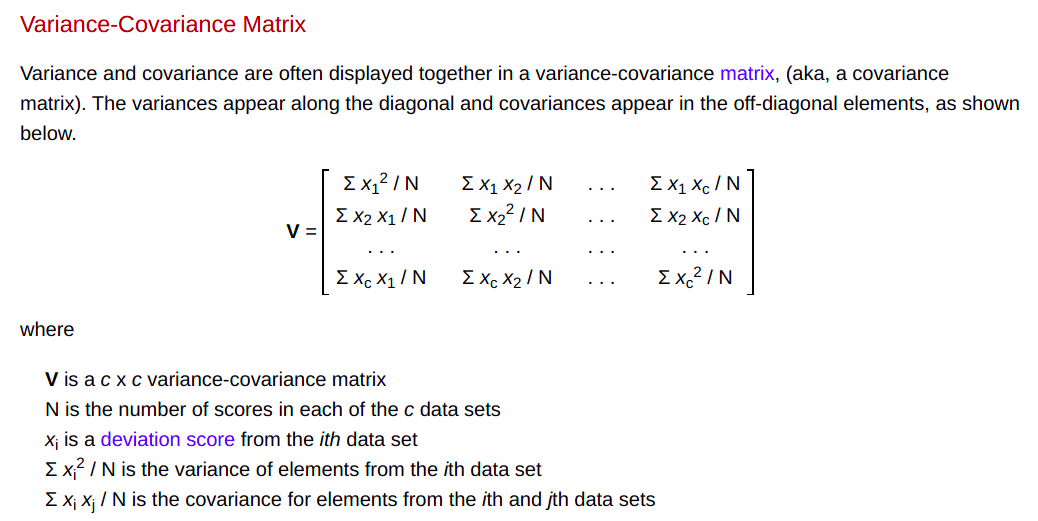
Variance – variability of data = average squared deviation from the mean (Var(X) = Σ (Xi-mean)^2/N)
Covariance - extent to which corresponding elements from two sets of ordered data move in the same direction ( Cov(X,Y) = Σ (Xi-X mean) (Yi-Y mean) / N) )
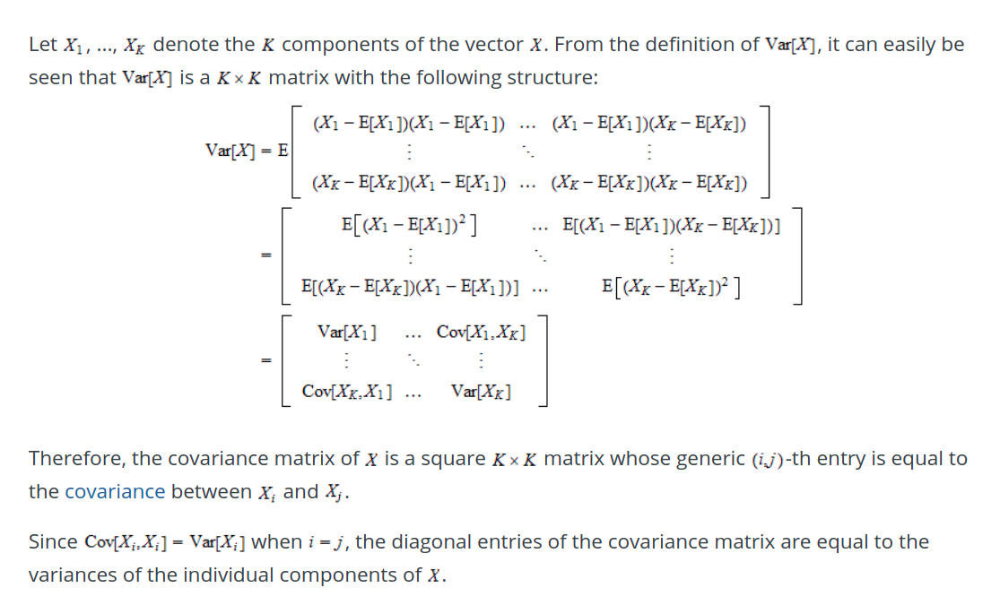
Covariance matrix
Explanation 1
|
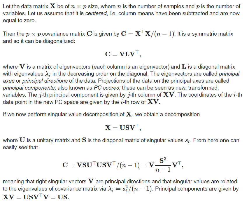
Explanation 2
|
More on LDA:
S. Raschka's ML book which I bought and his article here
SVD
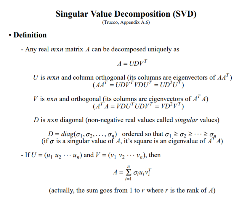


PCA vs. SVD
Usage:
Dimensionality reduction - keeping only n significant eigenvalues
Data compression - taking the n largest singular values AA, replacing the rest with zero (to form Σ′), and recomputing UΣ′VT gives you the probably-best n-rank approximation to the matrix.
Solving linear equations
PCA and SVD are closely related and decompose any rectangular matrix. To calculate their relationship, perform SVD on covariance matrix C:
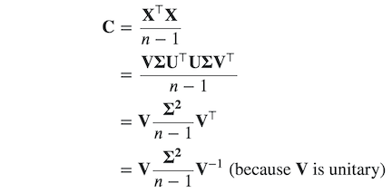
Hence, the relationship between eigenvalues and singular values is:
 It suggests that we can actually perform PCA using SVD, or vice versa. In fact, most implementations of PCA actually perform SVD under the hood rather than doing eigen decomposition on the covariance matrix because SVD can be much more efficient and is able to handle sparse matrices. In addition, there are reduced forms of SVD which are even more economic to compute.
Notes from Andrew Ng’s course (TO PROCESS AND ADD TO THE ABOVE)