Algorithm Analysis & Big-O · Coding Interview Guide

Challenges on this page

Introduction to Algorithm Analysis and Big O
Big O Notation
Big O Examples
Big O for Python Data Structures

01Introduction to Algorithm Analysis and Big O

Source notebook: Introduction to Algorithm Analysis and Big O .ipynb

Introduction to Algorithm Analysis and Big O

In this lecture we will discuss how to analyze Algorithms and why it is important to do so!

Why analyze algorithms?

Before we begin, let's clarify what an algorthim is. In this course, an algorithm is simply a procedure or formula for solving a problem. Some problems are famous enough that the algorithms have names, as well as some procdures being common enough that the algorithm associated with it also has a name. So now we have a good question we need to answer:

** How do analyze algorithms and how can we compare algorithms against each other? **

Imagine if you and a friend both came up with functions to sum the numbers from 0 to N. How would you compare the functions and algorithms within the functions? Let's say you both cam up with these two seperate functions:

Python

# First function (Note the use of xrange since this is in Python 2)
def sum1(n):
    '''
    Take an input of n and return the sum of the numbers from 0 to n
    '''
    final_sum = 0
    for x in xrange(n+1): 
        final_sum += x
    
    return final_sum

Python

sum1(10)

Output

Python

def sum2(n):
    """
    Take an input of n and return the sum of the numbers from 0 to n
    """
    return (n*(n+1))/2

Python

sum2(10)

Output

You'll notice both functions have the same result, but completely different algorithms. You'll note that the first function iteratively adds the numbers, while the second function makes use of: $$ \sum_{i=0}^{n} {i} = \frac{n(n+1)}{2} $$

So how can we objectively compare the algorithms? We could compare the amount of space they take in memory or we could also compare how much time it takes each function to run. We can use the built in %timeit magic function in jupyter to compare the time of the functions. The %timeit magic in Jupyter Notebooks will repeat the loop iteration a certain number of times and take the best result. Check out the link for the documentation.

Let's go ahead and compare the time it took to run the functions:

Python

%timeit sum1(100)

Output

The slowest run took 5.15 times longer than the fastest. This could mean that an intermediate result is being cached 
100000 loops, best of 3: 4.86 µs per loop

Python

%timeit sum2(100)

Output

The slowest run took 16.54 times longer than the fastest. This could mean that an intermediate result is being cached 
10000000 loops, best of 3: 173 ns per loop

We can see that the second function is much more efficient! Running at a much faster rate than the first. However, we can not use "time to run" as an objective measurement, because that will depend on the speed of the computer itself and hardware capabilities. So we will need to use another method, Big-O!

In the next lecture we will discuss Big-O notation and why its so important!

02Big O Notation

Source notebook: Big O Notation.ipynb

Big O Notation

In this lecture we will go over how the syntax of Big-O Notation works and how we can describe algorithms using Big-O Notation!

We previously discussed the functions below:

Python

# First function (Note the use of xrange since this is in Python 2)
def sum1(n):
    '''
    Take an input of n and return the sum of the numbers from 0 to n
    '''
    final_sum = 0
    for x in xrange(n+1): 
        final_sum += x
    
    return final_sum

Python

def sum2(n):
    """
    Take an input of n and return the sum of the numbers from 0 to n
    """
    return (n*(n+1))/2

Now we want to develop a notation to objectively compare the efficiency of these two algorithms. A good place to start would be to compare the number of assignments each algorithm makes.

The original sum1 function will create an assignment n+1 times, we can see this from the range based function. This means it will assign the final_sum variable n+1 times. We can then say that for a problem of n size (in this case just a number n) this function will take 1+n steps.

This n notation allows us to compare solutions and algorithms relative to the size of the problem, since sum1(10) and sum1(100000) would take very different times to run but be using the same algorithm. We can also note that as n grows very large, the +1 won't have much effect. So let's begin discussing how to build a syntax for this notation.

Now we will discuss how we can formalize this notation and idea.

Big-O notation describes how quickly runtime will grow relative to the input as the input get arbitrarily large.

Let's examine some of these points more closely:

Remember, we want to compare how quickly runtime will grows, not compare exact runtimes, since those can vary depending on hardware.
Since we want to compare for a variety of input sizes, we are only concerned with runtime grow relative to the input. This is why we use n for notation.
As n gets arbitrarily large we only worry about terms that will grow the fastest as n gets large, to this point, Big-O analysis is also known as asymptotic analysis

As for syntax sum1() can be said to be O(n) since its runtime grows linearly with the input size. In the next lecture we will go over more specific examples of various O() types and examples. To conclude this lecture we will show the potential for vast difference in runtimes of Big-O functions.

Runtimes of Common Big-O Functions

Here is a table of common Big-O functions:

Big-O	Name
1	Constant
log(n)	Logarithmic
n	Linear
nlog(n)	Log Linear
n^2	Quadratic
n^3	Cubic
2^n	Exponential

Now let's plot the runtime versus the Big-O to compare the runtimes. We'll use a simple matplotlib for the plot below. (Don't be concerned with how to use matplotlib, that is irrelevant for this part).

Python

from math import log
import numpy as np
import matplotlib.pyplot as plt
%matplotlib inline
plt.style.use('bmh')

# Set up runtime comparisons
n = np.linspace(1,10,1000)
labels = ['Constant','Logarithmic','Linear','Log Linear','Quadratic','Cubic','Exponential']
big_o = [np.ones(n.shape),np.log(n),n,n*np.log(n),n**2,n**3,2**n]

# Plot setup
plt.figure(figsize=(12,10))
plt.ylim(0,50)

for i in range(len(big_o)):
    plt.plot(n,big_o[i],label = labels[i])


plt.legend(loc=0)
plt.ylabel('Relative Runtime')
plt.xlabel('n')

Output

<matplotlib.text.Text at 0x10cec7cd0>

Output

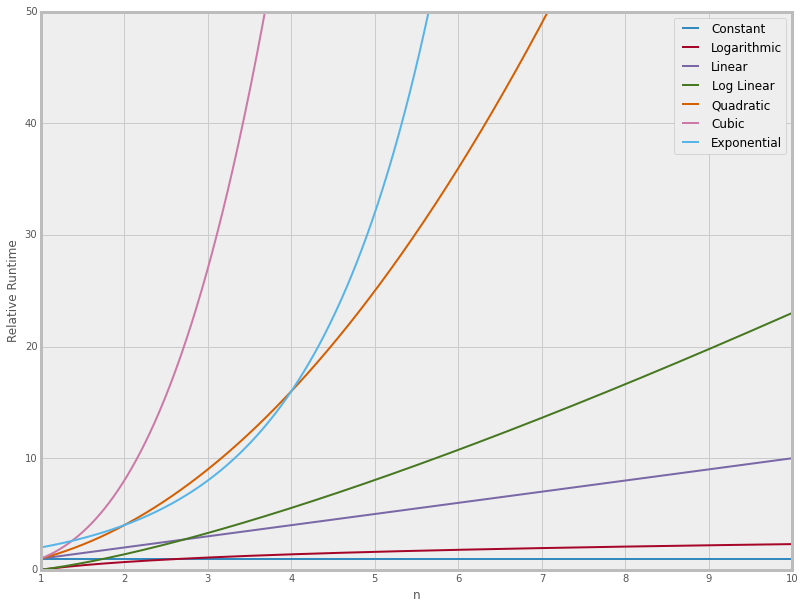
Note how much of a difference a Big-O efficiency can make for the same n value against the projected runtime! Clearly we want to choose algorithms that stay away from any exponential, quadratic, or cubic behavior!

In the next lecture we will learn how to properly denote Big-O and look at examples of various problems and calculate the Big-O of them!

03Big O Examples

Source notebook: Big O Examples .ipynb

Big O Examples

In the first part of the Big-O example section we will go through various iterations of the various Big-O functions. Make sure to complete the reading assignment!

Let's begin with some simple examples and explore what their Big-O is.

O(1) Constant

Python

def func_constant(values):
    '''
    Prints first item in a list of values.
    '''
    print values[0]
    
func_constant([1,2,3])

Output

Note how this function is constant because regardless of the list size, the function will only ever take a constant step size, in this case 1, printing the first value from a list. so we can see here that an input list of 100 values will print just 1 item, a list of 10,000 values will print just 1 item, and a list of n values will print just 1 item!

O(n) Linear

Python

def func_lin(lst):
    '''
    Takes in list and prints out all values
    '''
    for val in lst:
        print val
        
func_lin([1,2,3])

Output

1
2
3

This function runs in O(n) (linear time). This means that the number of operations taking place scales linearly with n, so we can see here that an input list of 100 values will print 100 times, a list of 10,000 values will print 10,000 times, and a list of n values will print n times.

O(n^2) Quadratic

Python

def func_quad(lst):
    '''
    Prints pairs for every item in list.
    '''
    for item_1 in lst:
        for item_2 in lst:
            print item_1,item_2
            
lst = [0, 1, 2, 3]

func_quad(lst)

Output

Note how we now have two loops, one nested inside another. This means that for a list of n items, we will have to perform n operations for every item in the list! This means in total, we will perform n times n assignments, or n^2. So a list of 10 items will have 10^2, or 100 operations. You can see how dangerous this can get for very large inputs! This is why Big-O is so important to be aware of!

Calculating Scale of Big-O

In this section we will discuss how insignificant terms drop out of Big-O notation.

When it comes to Big O notation we only care about the most significant terms, remember as the input grows larger only the fastest growing terms will matter. If you've taken a calculus class before, this will reminf you of taking limits towards infinity. Let's see an example of how to drop constants:

Python

def print_once(lst):
    '''
    Prints all items once
    '''
    for val in lst:
        print val

Python

print_once(lst)

Output

The print_once() function is O(n) since it will scale linearly with the input. What about the next example?

Python

def print_3(lst):
    '''
    Prints all items three times
    '''
    for val in lst:
        print val
        
    for val in lst:
        print val
        
    for val in lst:
        print val

Python

print_3(lst)

Output

We can see that the first function will print O(n) items and the second will print O(3n) items. However for n going to inifinity the constant can be dropped, since it will not have a large effect, so both functions are O(n).

Let's see a more complex example of this:

Python

def comp(lst):
    '''
    This function prints the first item O(1)
    Then is prints the first 1/2 of the list O(n/2)
    Then prints a string 10 times O(10)
    '''
    print lst[0]
    
    midpoint = len(lst)/2
    
    for val in lst[:midpoint]:
        print val
        
    for x in range(10):
        print 'number'

Python

lst = [1,2,3,4,5,6,7,8,9,10]

comp(lst)

Output

1
1
2
3
4
5
number
number
number
number
number
number
number
number
number
number

So let's break down the operations here. We can combine each operation to get the total Big-O of the function:

$$O(1 + n/2 + 10)$$

We can see that as n grows larger the 1 and 10 terms become insignificant and the 1/2 term multiplied against n will also not have much of an effect as n goes towards infinity. This means the function is simply O(n)!

Worst Case vs Best Case

Many times we are only concerned with the worst possible case of an algorithm, but in an interview setting its important to keep in mind that worst case and best case scenarios may be completely different Big-O times. For example, consider the following function:

Python

def matcher(lst,match):
    '''
    Given a list lst, return a boolean indicating if match item is in the list
    '''
    for item in lst:
        if item == match:
            return True
    return False

Python

lst

Output

[1, 2, 3, 4, 5, 6, 7, 8, 9, 10]

Python

matcher(lst,1)

Output

True

Python

matcher(lst,11)

Output

False

Note that in the first scenario, the best case was actually O(1), since the match was found at the first element. In the case where there is no match, every element must be checked, this results in a worst case time of O(n). Later on we will also discuss average case time.

Finally let's introduce the concept of space complexity.

Space Complexity

Many times we are also concerned with how much memory/space an algorithm uses. The notation of space complexity is the same, but instead of checking the time of operations, we check the size of the allocation of memory.

Let's see a few examples:

Python

def printer(n=10):
    '''
    Prints "hello world!" n times
    '''
    for x in range(n):
        print 'Hello World!'

Python

printer()

Output

Hello World!
Hello World!
Hello World!
Hello World!
Hello World!
Hello World!
Hello World!
Hello World!
Hello World!
Hello World!

Note how we only assign the 'hello world!' variable once, not every time we print. So the algorithm has O(1) space complexity and an O(n) time complexity.

Let's see an example of O(n) space complexity:

Python

def create_list(n):
    new_list = []
    
    for num in range(n):
        new_list.append('new')
    
    return new_list

Python

print create_list(5)

Output

['new', 'new', 'new', 'new', 'new']

Note how the size of the new_list object scales with the input n, this shows that it is an O(n) algorithm with regards to space complexity.

Thats it for this lecture, before continuing on, make sure to complete the homework assignment below:

Homework Assignment

Your homework assignment after this lecture is to read the fantastic explanations of Big-O at these two sources:

04Big O for Python Data Structures

Source notebook: Big O for Python Data Structures.ipynb

Big O for Python Data Structures

In this lecture we will go over the Big O of built-in data structures in Python: Lists and Dictionaries.

Lists

In Python lists act as dynamic arrays and support a number of common operations through methods called on them. The two most common operations performed on a list are indexing and assigning to an index position. These operations are both designed to be run in constant time, O(1).

Let's imagine you wanted to test different methods to construct a list that is [0,1,2...10000]. Let go ahead and compare various methods, such as appending to the end of a list, concatenating a list, or using tools such as casting and list comprehension.

For example:

Python

def method1():
    l = []
    for n in xrange(10000):
        l = l + [n]

def method2():
    l = []
    for n in xrange(10000):
        l.append(n)

def method3():
    l = [n for n in xrange(10000)]

def method4():
    l = range(10000) # Python 3: list(range(10000))

Let's now test these methods using the timeit magic function:

Python

%timeit method1()
%timeit method2()
%timeit method3()
%timeit method4()

Output

10 loops, best of 3: 162 ms per loop
1000 loops, best of 3: 820 µs per loop
1000 loops, best of 3: 307 µs per loop
10000 loops, best of 3: 77.7 µs per loop

We can clearly see that the most effective method is the built-in range() function in Python!

It is important to keep these factors in mind when writing efficient code. More importantly begin thinking about how we are able to index with O(1). We will discuss this in more detail when we cover arrays general. For now, take a look at the table below for an overview of Big-O efficiencies.

Table of Big-O for common list operations

** Please note, in order to see this table, you may need to download this .ipynb file and view it locally, sometimes GitHub or nbveiwer have trouble showing the HTML for it... **

Operation	Big-O Efficiency
index []	O(1)
index assignment	O(1)
append	O(1)
pop()	O(1)
pop(i)	O(n)
insert(i,item)	O(n)
del operator	O(n)
iteration	O(n)
contains (in)	O(n)
get slice [x:y]	O(k)
del slice	O(n)
set slice	O(n+k)
reverse	O(n)
concatenate	O(k)
sort	O(n log n)
multiply	O(nk)

Dictionaries

Dictionaries in Python are an implementation of a hash table. They operate with keys and values, for example:

Python

d = {'k1':1,'k2':2}

Python

d['k1']

Output

Something that is pretty amazing is that getting and setting items in a dictionary are O(1)! Hash tables are designed with efficiency in mind, and we will explore them in much more detail later on in the course as one of the most important data structures to undestand. In the meantime, refer to the table below for Big-O efficiencies of common dictionary operations:

Operation	Big-O Efficiency
copy	O(n)
get item	O(1)
set item	O(1)
delete item	O(1)
contains (in)	O(1)
iteration	O(n)

Conclusion

By the end of this section you should have an understanding of how Big-O is used in Algorithm analysis and be able to work out the Big-O of an algorithm you've developed. Get ready, there's a quiz up next!