- UNIX
- ML At Scale
- Picking the Right Framework and Language
- Using the Right Processors: CPUs, GPUs, ASICs, and TPUs
- Data Collection and Warehousing
- Input Pipeline
- Model Training
- Distributed Machine Learning
- Other optimizations
- Resource utilization and monitoring
- Deploying and Real-world Machine Learning
- Causal Analysis (more general than A/B testing)
- 4 steps to conducting a cohort analysis
- GENERAL ML & DL REFERENCES
- INCORPORATE THE TOPICS BELOW
- CLASSICAL SUPERVISED LEARNING
- UNSUPERVISED LEARNING
- DEEP LEARNING CORE
- TRANSFER/MULTITASK/CONTINUAL/META/NAS
- REINFORCEMENT LEARNING & BANDITS
- DISTANCE METRICS
- DOMAIN-SPECIFIC ML
- EFFICIENCY & SYSTEMS
- EVALUATION & VALIDATION
- DATA & FEATURES
- DATASETS
- MLOPS & PRODUCTIONIZATION
- MATHEMATICS & THEORY
- PROJECT, PROCESS & ETHICS
- RECOMMENDER SYSTEMS & SEARCH
- REGULARIZATION & AUGMENTATION
- ROBUSTNESS/SECURITY/FAIRNESS/PRIVACY
- SPEECH & AUDIO
- OTHER / UNCATEGORIZED
- BAYESIAN & PROBABILISTIC
- TIME SERIES & FORECASTING
- CAUSALITY & UPLIFT
UNIX
Linux is a free, open-source OS. Used from web servers (90%) to cellphones (Andriod, iOS?). Flavors - Ubuntu, Red Hat (CentOS), Linux Mint, Debian, Fedora
Interactive terminal shell - executing administrative commands (file manipulation, package installation, and user management). GUI also
pwd - print working directory
ls - list content
cd - change directory
cd .. - go up
mkdir, rmdir - create / remove (empty) dir
cat filename - print content
less filename - print one page at a time
touch / rm filename - create / remove a file
rm - remove file or directory (rm -r: recursively w/files)
cp source destination - copy file
mv source destination - move file
nano filename - edit file (other editors vim, emacs)
man <command> - show manual for the command (OR <command> --help)
locate - find a file
sudo - SuperUser Do
tar zip/unzip
apt-get - install package
chmod - make a file executable or change permissions
File system is based on a directory tree: directories inside directories + files. Each user has a /home directory. There is a /root directory. File permissions - who can read and write certain files.
More at https://www.tutorialspoint.com/unix/index.htm
ML At Scale
Auto-scaler - when load increases or a model is run at a certain busy time. GCP compute engine can add virtual machines automatically.
Load balancer – distributes a set of tasks over a set of resources to make processing more efficient; optimizes response time and avoids unevenly overloading some compute nodes while other compute nodes are idle.
Article at https://www.codementor.io/blog/scalable-ml-models-6rvtbf8dsd
Picking the Right Framework and Language
Using the Right Processors: CPUs, GPUs, ASICs, and TPUs
Data Collection and Warehousing
Input Pipeline
I/O hardware are also important for machine learning at scale - the massive data for iterative perform computations is fetched from and stored by I/O devices and the input pipeline can quickly become a bottleneck if not optimized. Steps to consider:
1. Extraction
2. Transformation
3. Loading
Model Training
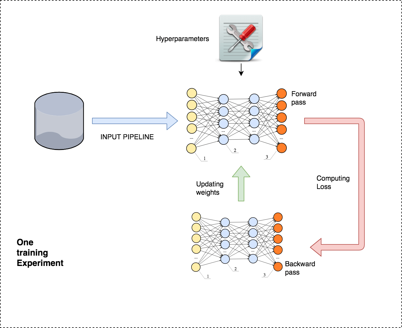
Feeding the data via the input pipeline, forward pass, computing loss, updating weight to minimize the loss. Let's decompose the computations performed in these steps into granular ones that can be run independently and aggregated later. After decomposition, leverage horizontal scaling of the systems to improve time, cost, and performance.
Decomposition of model training
Functional decomposition
Breaking the logic down to distinct and independent functional units, which can later be recomposed to get the results. "Model parallelism" in ML - split different parts of the model computations to different devices to execute them in parallel and speed up training.
Data decomposition
Data is divided into chunks, and multiple machines perform the same computations on different data chunks.
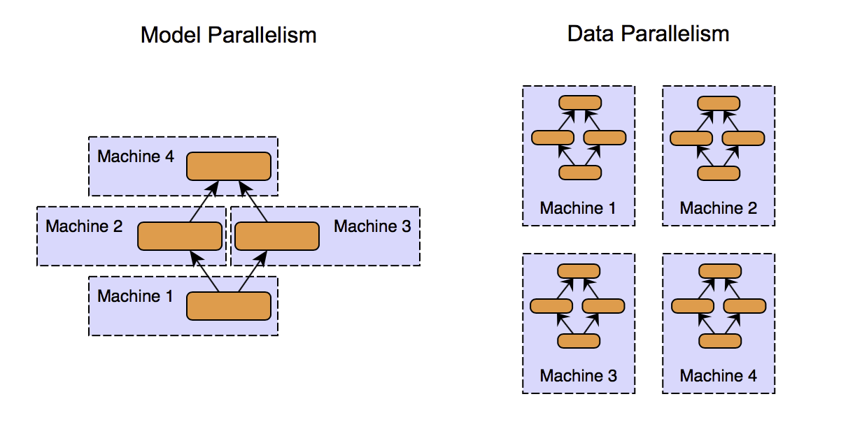
Example of both functional and data decomposition - training of an ensemble learning model like random forest => functional decomposition of model into individual DT trees + training individual trees as data parallelism.
Distributed Machine Learning
MapReduce
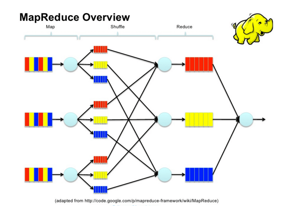
Parallelization of computations - "split-apply-combine" strategy. Map f(x) maps data to key-value pairs, shuffle groups similar key-value pairs, reduce aggregates key-value groups.
In MapReduce data is handled in a distributed, highly optimized manner on multiple workers (cluster of nodes) => scalability.
Components of distributed ML:
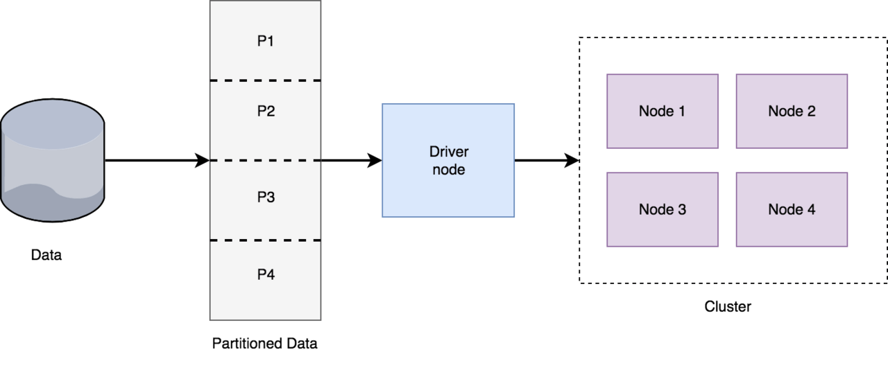
Data is partitioned, driver node assigns tasks to the nodes in the cluster who might have to communicate with each other (e.g. on gradients). Possible node arrangements: Async parameter server and Sync AllReduce.
Async parameter server architecture
Transmission of info between nodes is asynchronous:
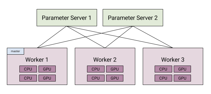
Single worker has multiple computing devices. Master’s role - driver. Workers communicate info (e.g. gradients) to parameter servers, update parameters (weights), pull latest parameters (weights) from parameter server. Drawback - delayed convergence, as workers can go out of sync.
Sync AllReduce architecture
Synchronous transmission of info between the cluster nodes:
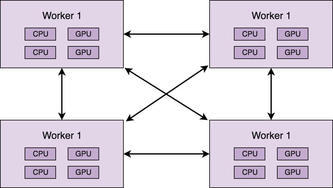
All workers must be synced before a new iteration; communication links must be fast (effective). There's no parameter server. More suited for fast hardware accelerators.
Some distributed ML frameworks provide high-level APIs for such arrangements.
Popular distributed ML frameworks
A distributed computation framework should do data handling / task distribution, provide fault tolerance, recovery, etc.
Open-source implementation of MapReduce - Apache Hadoop. Data stored in the Hadoop Distributed File System (HDFS), MapReduce API in multiple languages. Hadoop’s scheduler - YARN (Yet Another Resource Negotiator) which optimizes the scheduling of tasks to workers.
Apache Spark - immutable Resilient Distributed Datasets (RDDs) - core data structure to represent the data and perform faster in-memory computations on streaming and iterative workloads. Can use MapReduce or Mllib to write algos. Other aspects of Spark: Spark Core, data frames, the Spark Shell, Spark Streaming, Spark SQL, MLlib
Spark is very versatile in the sense that it can run as standalone cluster mode, on EC2, Hadoop YARN, Mesos, or Kubernetes. Multiple data sources can be used: HDFS, Apache Cassandra, Apache HBase, Apache Hive, many more.
Another framework - Apache Mahout for distributed linear-algebra computations, supports Spark engine. Easier to implement algorithms in Mahout if they not implemented in Spark’s MLlib.
Message Passing Interface (MPI) - another programming paradigm for parallel computing. More general, provides a standard for communication between processes by message-passing - more flexibility (and control) in inter-node communication in the cluster. Use case: smaller datasets or when more communication among decomposed tasks needed.
DL frameworks TensorFlow, MxNet, PyTorch have APIs for distributed computations by model and data parallelism.
There are higher-level frameworks like horovod and elephas built on top of these frameworks. It all boils down to what your use-case is and your level of abstraction.
Hyperparameter Optimization
HP optimization strategy to select the best (or approximately best) hyperparameters is important - the hyperparameter search space can be large, and it may not be practically feasible to try every combination.
For simpler algorithms like SVM, DTs, etc. - random search, Bayesian optimization, evolutionary optimization (distributed HP optimization: Ray and Hyperopt).
Other optimizations
Memory efficient backpropagation
There have been active research to diminish the linear scaling of NN with depth and batch size. Square root scaling w/slightly higher computation complexity: arXiv:1604.06174. Implemented in the Openai/gradient-checkpointing package for TensorFlow models.
Low numerical precision training
There is evidence that using lower numerical precision (16-bit for training, and 8-bit for inference instead of 32-bit floating point precision) may have minimal impact on accuracy. But, this can also lead to quantization noise, gradient underflow, imprecise weight updates, etc. See mixed precision training.
Other considerations
Lots of emerging techniques, but keep this in mind:
In many cases, metrics are not the only important thing. If it takes multiple additional training iterations to gain negligible improvements of the metrics.
Try not to reinvent the wheel and use transfer learning to fine-tune pre-trained models like GloVe vectors for sentiment or VGG-16 for images.
There isn't a one-technique-fits-all for solving scaling problems in ML - look for distributed versions of algorithms: Elastic SGD, Asynchronous SGD, etc. But not everything can be parallelized.
With ML at scale - tracking versions and history of the models is vital (architecture, HPs, how previous iterations performed, etc.) to make an intelligent choice.
Resource utilization and monitoring
Important for cost saving purposes.
Deploying and Real-world Machine Learning
How to serialize your model, separate the architecture (algorithm) and the coefficients (parameters), integrate a model inside an existing software or expose it to the web?
If expose it to the web:
execute a TF model in user's browser with TensorFlow.js, which is a WebGL based library for deploying/training ML models that also supports hardware acceleration. No back-end needed, but model is publically visible (weights) + inference time depends on the client's machine;
if back-end with API - typical webserver with a load balancer (or a queue mechanism) and multiple workers (consumers).
Serverless architecture (AWS lambda) for running inference, hides operational complexity, pay-per-execution, but has a cold start time of a few seconds (for every execution request).
Amazon SageMaker, Google Cloud ML, Azure ML - auto-scaling, HP autotuning, easy deploy with rolling updates, well-defined pipelines. Downside - ecosystem lock-in (less flexibility) and a higher cost.
Other distributed computations aspects: graph processing algorithms (pagerank / shortest path), matrix factorization
Note: there are more than enough references below to study causal inference / analysis. Plus downloaded books on causal inference and downloaded articles for causal NLP!
Causal Analysis (more general than A/B testing)
If X = new feature / product / drug and Y is its outcome, we always want to know “Does X drive Y?” or “If I do X, will Y happen?” (not the same as “if X happens, then Y will happen” because we force X to happen, while in the second case, X is happening spontaneously).
E.g., a) website owner wants to know if a new web page design leads to a higher click-through rate / sale; b) clinical researcher - if a new drug promotes better health. In marketing this helps isolate the effects of a specific campaign on targeted clients, getting rid of potential selection bias.
Causality is more informative than correlation. Raw correlation between X and Y is NOT enough to establish the causal relationships.
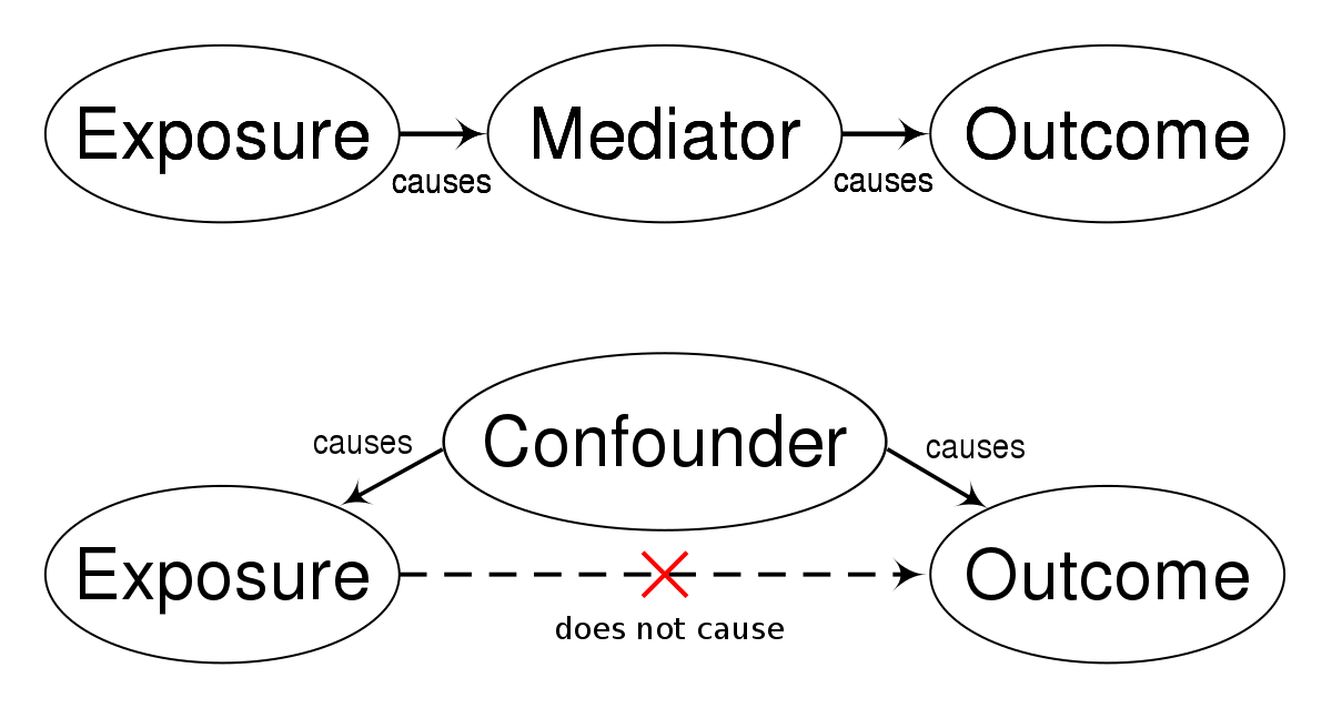
Complicating factor - set of features called Confounding Variables that affect both X and Y by imposing spurious correlations. (visitor geolocation, gender, age and interest affect the use of the new feature and the outcome of sales revenue) => need to isolate the effect of the new web page design (X) on the sales revenue (Y) while controlling for these confounding variables.
Two main types of causal studies:
Observational study - observe and collect data (e.g., X and Y).
Experimental study - randomly impose treatment to a group, while the other group doesn’t receive the treatment, to investigate the causal relationship between the treatment and the outcome variable. Randomization and intervention (the actual doing of something that will cause the effect) make experimental studies different from observational studies.
Randomized controlled trials (RCTs) are the gold standard for measuring causality. In our marketing campaign example - randomly split population into 2 groups: one receives the campaign (group A), and the other doesn’t (group B) (how new medicines are tested).
Brief Idea
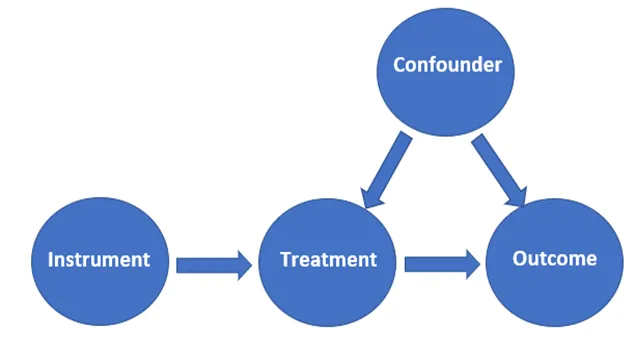
Confounder: confounding variable / confounding factor - influences both the dependent variable and independent variable, causing a spurious association.
Treatment: has a direct effect on outcome.
Instrument: Instrument variable is the one that has direct causal effect on the treatment variable but not on the outcome variable.
Outcome: It is the one that depends or gets influenced by the input feature/independent feature.
Treatment effect: It is the impact created by the treatment variable on the outcome variable. It highlights the difference between potential outcomes when treated vs when not treated.
ATE – average treatment effect. It is the average difference between the potential outcome when treated vs when not treated = global treatment (at a population level). When the effect is calculated only for the treatment group, it is known as ATT (Average treatment effect on treated). When it is calculated only for the control group, it is known as ATC (Average treatment effect on control).
ITE – Individual treatment effect - at individual level = does treatment affects the outcome of an individual unit positively or negatively.
CATE – Conditional average treatment effect - at the subgroup level = average individual treatment effect of the subgroup. Customer segmentation is done based on CATE value. It is also known as the heterogeneous treatment effect.
A/B Testing as a Tool for Causal Inference
The A/B test (a.k.a, Randomized Controlled Trial) is perhaps the most accurate tool to investigate causality. Causal inference is a process by which a causal connection is established based on evidence. In A/B testing this happens through hypothesis testing, usually in the form of a Null Hypothesis Statistical Test.
Definitions
Spurious correlation - two or more variables are associated, but not causally related, due to either coincidence or the presence of a certain third, unseen factor
Counterfactual explanation describes a causal situation in the form: “If X had not occurred, Y would not have occurred”. For example: “If I hadn’t taken a sip of this hot coffee, I wouldn’t have burned my tongue”. Event Y is that I burned my tongue; cause X is that I had a hot coffee. This is like imagining a hypothetical reality that contradicts the observed facts (for example, a world in which I have not drunk the hot coffee), hence the name “counterfactual”.
Cohort Analysis (to be summarized)
Cohort analysis is a type of behavioral analytics in which you take a group of users, and analyze their usage patterns based on their shared traits to better track and understand their actions. A cohort is simply a group of people with shared characteristics = customer churn analysis.
To get directly at churn reduction, you need to first diagnose your product's specific problems. Then, make adjustments. Cohort analysis allows you to ask more specific, targeted questions and make informed product decisions that will reduce churn and drastically increase revenue. You could also call it customer churn analysis.
The 2 most common types of cohorts are:
Acquisition cohorts: Groups divided based on when they signed up for your product. Typically, the shared characteristics of this group of users offers an opportunity to measure retention and churn rates within a specific timeframe.
Behavioral cohorts: Groups divided based on their behaviors and actions in your product. This type allows you to view your active users in different demographics and with different behavioral patterns.
Acquisition cohorts help you understand when an action is taking place, but behavioral cohorts are best for discovering and understanding churn rates, as they tell you why a user has taken an action.
5 benefits of cohort analysis
Cohort analysis is a valuable tool for anyone looking to gain a deeper understanding of their customers and why they make certain choices in your app. Here are some of the benefits of conducting cohort analysis:
Determine business health. A great indicator of a healthy business is increasing revenue even if you aren’t acquiring new customers. Jonathan Parisot, co-founder and CEO at Actiondesk, says that cohort analysis "can help you determine which cohorts/groups of customers are contributing the most to revenue." This, in turn, allows you to focus on upselling other products or services to them.
Understand customers better. Cohort analysis allows businesses to gain a deeper understanding of their customers by tracking their behavior over a period of time. This can help you identify patterns and trends that may not be immediately apparent from looking at vanity metrics.
Enhanced customer segmentation. By dividing user groups and creating specific cohorts, businesses can create more targeted and effective marketing campaigns and offer personalized customer experiences.
Increased customer retention. Jonathan also adds that cohort analysis helps by analyzing retention rates and identifying potential churn risks. With this information in hand, you can take proactive steps to improve customer experiences.
Optimize your app for increased interest. You can use cohort analysis to optimize the user experience and increase customer lifetime value by identifying trends and patterns in the customer lifecycle.
4 steps to conducting a cohort analysis
1. Look at when users churn
Your users are the ones with mouths, but the timeline is going to tell you more about your churn problem than they ever will. If you find out when the churn happens, you can figure out what’s happening around that time to cause it.
But how do you establish the timeline in the first place? By performing an acquisition cohort analysis.
In this case, you need to create a cohort chart. You need your various cohorts, as well as the number of users for each and a column for each day of the period you’re analyzing.
Like this:
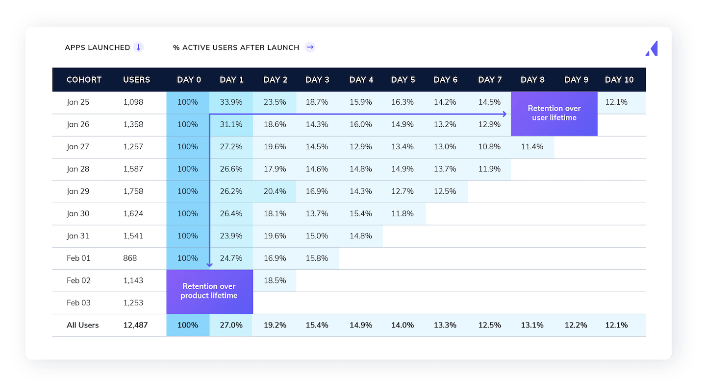
As you can see, the cells under each day show the portion of the original cohort for that row that you’ve retained on that day. Nice.
A couple of things to remember as you’re setting up your acquisition cohort analysis:
Time period: Use time periods that make sense for the age of your app and user base. Days typically work well, but in some cases, weeks and months make sense, too.
Focused scope: The more you zoom out on your retention, the harder it is to see the details that will really tell you what’s going wrong. If you need to, break your analysis into multiple analyses focused on your typical user retention periods: early, middle and late.
2. Find the sticky features
With your trusty acquisition cohort analysis and timeline in hand (who and what), the next step is the analysis (why). Look for the big drop-offs and make a note of them. Ask yourself what happened on those drop-off days.
Imagine you’re seeing users drop off by 23% on day 3 (yikes). What happens on day 3? Are you asking them to sync their data (for example)? If the answer is yes, you’ve found the problem. Maybe not the problem, but a problem you can solve nonetheless.
Your analyses will likely be more complex. In fact, you’ll probably need to apply this analysis to all of your app’s core features. Here’s what you should not do: See how app engagement in the first 30 days correlates with churn. Why? Because that information tells you nothing about what to change.
Here’s a better idea: How does the completion of an app onboarding checklist correlate with churn? In other words, keep it specific. Which specific features are sticky for your users? That’s what you need to find out.
3. Compare behavioral cohorts
Wouldn’t it be great if the problem was always a single feature? Sure. But that’s almost never the case.
It’s usually a combination of features and behaviors that influences cohort churn. For example, those who complete the onboarding checklist in your app may be much less likely to churn when you ask them to sync their data than those who didn’t.
That’s just one extra layer, but remember—there are dozens of layers to consider. How do you do that? By comparing your behavioral cohorts. If you’re handy with pivot tables and conditional formatting and have a lot of time on your hands, you can do it in a spreadsheet.
Or you can use one of the many tools designed to streamline the churn cohort analysis process. Amplitude, for examplitude, is purpose-built for creating and comparing behavioral cohorts in a flash.
(Here’s a quick guide on how to use Amplitude for cohort analysis.)
As you get deep into the data, don’t forget your purpose. You’re trying to find the combinations of behaviors and features that are influencing retention—positively or negatively. That means you need to be analyzing this stuff in a way that spits out hypotheses ripe for the testing.
4. Iterate, rinse, and repeat
Test, test and test some more.
Your gut feeling that you need to add some reminders about the checklist to promote e.g. the best user onboarding experiences may be exactly right. That’s great, but test it so you can back it up with data.
And if you test a change to your app that improves retention, don’t stop there. You should have at least a handful of other hypotheses to test. Test those, too.
Why? Because you may find that other changes reduce churn even more than the first one you tested. Be thorough. Take your time. Iterate it, rinse it, repeat it until you’ve solved the problem you came to solve.
References
Cohort analysis (incl. An example): https://www.appcues.com/blog/cohort-analysis#:~:text=Cohort%20analysis%20is%20a%20type,of%20people%20with%20shared%20characteristics.
A comprehensive guide to causal analysis (non-NLP): https://www.latentview.com/blog/a-comprehensive-guide-to-causal-analysis/
Causal inference (Part 1 of 3): Understanding the fundamentals - https://medium.com/data-science-at-microsoft/causal-inference-part-1-of-3-understanding-the-fundamentals-816f4723e54a
Python packages for causal inference: https://towardsdatascience.com/4-python-packages-to-learn-causal-analysis-9a8eaab9fdab
Python example of causal inference: https://towardsdatascience.com/implementing-causal-inference-a-key-step-towards-agi-de2cde8ea599
Beginner’s Guide to Cohort Analysis: https://www.appcues.com/blog/cohort-analysis#:~:text=Cohort%20analysis%20is%20a%20type,of%20people%20with%20shared%20characteristics.
Causal inference using NLP, main article with links to previous fundamental articles: https://towardsdatascience.com/causal-inference-using-natural-language-processing-da0e222b84b
Causal inference for NLP (downloaded article): https://arxiv.org/abs/2109.00725
Papers about Causal Inference and Language! https://github.com/causaltext/causal-text-papers
Causality for NLP Reading List (tons of papers / links): https://github.com/zhijing-jin/Causality4NLP_Papers
GENERAL ML & DL REFERENCES
Python notebooks covering the entire text of “Understanding Deep Learning” - multiple practical examples in code! (book downloaded in Recent ML Downloads on my laptop). Another link here.
INCORPORATE THE TOPICS BELOW
Most common ML Interview Qs (incorporate later)
CLASSICAL SUPERVISED LEARNING
AdaBoost
Bagging
Blending
CatBoost
Class weighting
Complement Naive Bayes
Cost-sensitive learning
Decision Trees
Decision trees (CART)
Distance-weighted k-NN
Elastic Net
Elastic Net regression
ExtraTrees
Focal loss for imbalance
GBDT
GLMs (Poisson, Gamma, Tweedie)
Generalized Linear Models (GLMs)
GentleBoost
Gradient Boosting
Gradient Boosting Machines
Imbalance handling (SMOTE, ADASYN, Borderline-SMOTE, SMOTE-NC)
Kernel SVMs
Kernel trick
LARS
Lasso regression
LightGBM
Linear regression
Logistic regression
LogitBoost
Multinomial logistic regression
Naive Bayes
Oblique decision trees
One-class SVM
Ordinal regression
Ordinary Least Squares (OLS)
Polynomial kernel
Probit regression
Pruning strategies
RBF kernel
Radial Basis Function (RBF) kernel
Random Forests
Ridge regression
Rotation Forests
SVM (kernel)
SVM (linear)
SVR
Sigmoid kernel
Softmax regression
Stacking
String kernels
Subbagging
Support Vector Machines (SVM)
Support Vector Regression (SVR)
Threshold moving
XGBoost
k-Nearest Neighbors (k-NN)
ν-SVM
UNSUPERVISED LEARNING
Affinity propagation
BIRCH
CURE clustering
DBSCAN
Dictionary learning
Divisive clustering
Expectation-Maximization (EM)
Factor Analysis
Gaussian Mixture Models (GMM)
HDBSCAN
HLLE
Hierarchical Dirichlet Process (HDP)
Hierarchical clustering
Hierarchical clustering (agglomerative)
Hierarchical clustering (divisive)
ICA (Independent Component Analysis)
Incremental PCA
Independent Component Analysis (ICA)
Isolation Forest
Isomap
Kernel Density Estimation (KDE)
Kernel PCA
LLE (Locally Linear Embedding)
Laplacian Eigenmaps
Latent Dirichlet Allocation (LDA topic model)
Local Outlier Factor (LOF)
Locally Linear Embedding (LLE)
Matrix factorization
Matrix factorization (SVD/ALS/NMF)
Mean shift clustering
Mini-batch k-Means
NMF (Non-negative Matrix Factorization)
Non-negative Matrix Factorization (NMF)
OPTICS
One-class SVM (anomaly detection)
PCA (Principal Component Analysis)
Parzen windows
Probabilistic Latent Semantic Analysis (PLSA)
Randomized PCA
Robust covariance estimation
Robust covariance outlier detection
Sparse PCA
Spectral clustering
Tensor factorization
Topic models (PLSA, LDA, HDP)
UMAP
k-Means
k-Means++
k-Medians
k-Medoids (PAM)
t-SNE
DEEP LEARNING CORE
Artificial neural networks
Backpropagation
Absolute positional encodings
Chain rule for backprop
Perceptron
Multi-layer perceptron (MLP)
Guardrail metrics
Dense connections
Label smoothing for classification
Mixed precision training (FP16/BF16)
Neuron interpretability
Phi-2
Power analysis for A/B tests
Heterogeneous treatment effect analysis in A/B
DenseNet
EfficientNet
Skip connections
Weight initialization (Xavier/Glorot, He initialization)
Teacher‚ student training
Residual Connections (Skip Connections)
Shortcuts in neural networks: the input of a layer bypasses intermediate layers and is added directly to the output - address the vanishing gradient problem and help train very deep networks by ensuring gradients can flow backward more effectively.
Stabilizes training of deep models
Improves convergence speed.
Enables construction of very deep architectures (e.g., ResNet with hundreds of layers)
Mechanism: Instead of learning the full mapping H(x) residual networks learn the residual function F(x)=H(x)−x. The final output is y=F(x)+x.
Dense connections
GRU
Highway networks
Kaiming initialization
Knowledge distillation
LSTM
Label smoothing for classification
Mixed precision training (FP16/BF16)
RNN
Teacher‚ student training
Weight initialization
Weight initialization (Xavier/Glorot, He initialization)
TRANSFER/MULTITASK/CONTINUAL/META/NAS
Adapters
Adversarial domain adaptation (DANN)
Concept shift adaptation
Continual learning: class-incremental, task-incremental
Covariate shift adaptation
DARTS
Domain adaptation
Domain adaptation (unsupervised, supervised)
Dynamic architectures for continual learning
ENAS
EWC (Elastic Weight Consolidation)
Elastic Weight Consolidation (EWC)
Evolutionary NAS
Experience replay buffers
Feature extraction transfer learning
Fine-tuning
GradNorm
Gradient-based NAS
Hard parameter sharing
Label shift adaptation
Low-Rank Adaptation (LoRA)
MAML
MAML (Model-Agnostic Meta-Learning)
Matching networks
Memory-augmented networks
Memory-augmented networks (NTM, DNC)
Meta-learning
Multitask learning
Multitask learning (hard parameter sharing)
Multitask learning (soft parameter sharing)
Neural Architecture Search (NAS)
Once-for-All networks
Online learning
Parameter Efficient Fine-Tuning (PEFT)
Progressive networks
Prototypical networks
ProxylessNAS
RL-based NAS
Reinforcement learning NAS
Relation networks
Reptile
Reptile algorithm
SI (Synaptic Intelligence)
Sim-to-real transfer
Soft parameter sharing
Task uncertainty weighting
Task weighting strategies
Transfer learning (feature extraction)
Transfer learning (fine-tuning)
Weight-sharing NAS
Zero-Cost NAS
REINFORCEMENT LEARNING & BANDITS
A2C
A3C
AIRL
Actor-Critic methods
Actor–Critic
AlphaZero
BCQ
BEAR
Bandit learning
Behavior cloning
Bellman equations
CQL (Conservative Q-Learning)
Combinatorial bandits
Contextual bandits
Curriculum in RL
DAgger (Dataset Aggregation)
DDPG
DQN
Decision Transformer
Deep Q-Network (DQN)
Distributional DQN (C51)
Double DQN
Dueling DQN
Dueling bandits
Dyna
Dynamic programming for RL
EXP3
EXP4
Epsilon-greedy exploration
Expected SARSA
Experience replay
Exploration strategies (epsilon-greedy, UCB, Thompson sampling, RND, ICM)
GAIL (Generative Adversarial Imitation Learning)
Generalized Advantage Estimation (GAE)
Hierarchical RL
IMPALA
IQL (Implicit Q-Learning)
IQN
Imitation learning
Intrinsic motivation in RL
KL-UCB
LinTS (Linear Thompson Sampling)
LinUCB
MBPO
MDP (Markov Decision Process)
Markov Decision Process (MDP)
Model-based RL
Monte Carlo methods in RL
MuZero
Multi-agent RL
Multi-armed bandit experiments
Multi-armed bandits
Noisy DQN
Non-stationary bandits
Off-policy evaluation
Offline RL
Option-critic
Options framework
PPO (KL-penalty)
PPO (clip)
Policy gradients
Policy iteration
Prioritized experience replay (PER)
Prioritized replay
Proximal Policy Optimization (PPO)
Q-learning
QR-DQN
REINFORCE
REINFORCE algorithm
Rainbow DQN
Reward design
Reward shaping
SAC
SARSA
Safe reinforcement learning
Self-play
Soft Actor-Critic (SAC)
Soft Q-learning
TD3
TRPO
Temporal difference learning (TD)
Thompson sampling
Thompson sampling (Beta–Bernoulli)
Trust Region Policy Optimization (TRPO)
UCB-Tuned
UCB1
Upper Confidence Bound (UCB)
Value iteration
DISTANCE METRICS
Bray‚ Curtis distance
Canberra distance
Chebyshev distance
Correlation distance
Cosine distance
Dynamic Time Warping (DTW)
Euclidean distance
Hamming distance
Jaccard distance
Mahalanobis distance
Manhattan distance
Minkowski distance
DOMAIN-SPECIFIC ML
Algorithmic trading ML
Autonomous driving (perception, planning, control)
Clinical NLP
Competing risks models
Credit scoring models
Demand forecasting
Differentiable simulators
Drug discovery ML
Finance ML (credit scoring, fraud detection, risk modeling)
Fraud detection
Genomics ML (variant calling, gene expression)
Geospatial ML (raster/vector data, satellite imagery)
Geospatial coordinate systems
Healthcare ML (PHI handling, de-identification)
Industrial IoT (predictive maintenance, anomaly detection)
Market impact models
Medical imaging (segmentation, detection)
Medical imaging models
PHI data handling
Physics-informed neural networks (PINNs)
Predictive maintenance
Raster data
Reinforcement learning for robotics
Retail/marketing ML (uplift modeling, MMM)
Risk modeling in finance
SLAM (simultaneous localization and mapping)
Scientific ML (physics-informed neural networks, surrogate modeling)
Scientific surrogate modeling
Sensor fusion
Spatiotemporal modeling
Spatiotemporal models
Survival analysis (Kaplan–Meier, Cox model)
Vector data
Visuomotor policies
EFFICIENCY & SYSTEMS
ANN algorithms (HNSW, IVF, IVF-PQ, IVF-OPQ, PQ, OPQ, LSH, DiskANN, Vamana, ScaNN)
Activation checkpointing
Apache Spark MLlib
Apache TVM
Approximate Nearest Neighbor (ANN) search
Asymmetric quantization
BLAS libraries (MKL, OpenBLAS)
Batching and scheduling
Batching strategies
CPU acceleration
CPU inference optimization
Caching strategies
Compilation and graph optimization (XLA, TVM, TensorRT, ONNX Runtime)
CuDNN
Dask
Data input pipelines (tf.data, PyTorch DataLoader)
Data parallelism
DeepSpeed
Distillation for edge
Dynamic routing
Early exiting
Edge inference
Expert parallelism (MoE)
FAISS
Fully Sharded Data Parallel (FSDP)
GPU acceleration
GPU inference optimization
Gradient checkpointing
HNSW
Horovod
IVF ANN
Knowledge distillation
Knowledge distillation (logit-based, feature-based)
LoRA
Lottery ticket hypothesis
Low-rank factorization
MKL library
Magnitude pruning
Megatron-LM
Mixed precision training
Model parallelism
Model pruning
Model pruning (structured)
Model pruning (unstructured)
NCCL
NVIDIA TensorRT
ONNX runtime
Offloading parameters to CPU/NVMe
Offloading to CPU/SSD
Optimized Product Quantization (OPQ16)
Optimized Product Quantization (OPQ32)
Optimized Product Quantization (OPQ64)
Optimized Product Quantization (OPQ8)
Per-channel quantization
Per-tensor quantization
Petastorm
Pipeline parallelism
Post-training quantization (PTQ)
Product Quantization
Pruning for edge
Quantization
Quantization for edge
Quantization-aware training (QAT)
Quantized inference
Ray
ScaNN ANN
Serverless inference
Structured pruning
Symmetric quantization
TPU acceleration
TPU-based training
Unstructured pruning
Vector databases
Vector databases (FAISS, HNSWlib, Annoy, Milvus, Qdrant, Weaviate, Pinecone, Chroma, Vespa, OpenSearch kNN)
WebDataset
XLA compiler
ZeRO optimization
cuBLAS
EVALUATION & VALIDATION
A/B testing
Adjusted Mutual Information (AMI)
Adjusted R-squared
Adjusted Rand Index (ARI)
BERTScore
Brier score
CRPS (Continuous Ranked Probability Score)
Calibration curves
Calinski–Harabasz index
Continuous Ranked Probability Score (CRPS)
Cost-sensitive evaluation
Counterfactual evaluation
Coverage
Davies-Bouldin index
Diebold–Mariano test
Dunn index
ECE (Expected Calibration Error)
Expected Calibration Error (ECE)
Fairness-aware evaluation
Forecasting metrics (MASE, WAPE, Pinball loss)
Hit rate
Interleaving tests
Intersection over Union (IoU)
Intra-list diversity
Isotonic regression calibration
Kernel Inception Distance (KID)
Log loss
MCE (Maximum Calibration Error)
MRR (Mean Reciprocal Rank)
McNemar’s test
Mean Absolute Percentage Error (MAPE)
Nested cross-validation
Normalized Mutual Information (NMI)
Novelty
Out-of-distribution testing
Permutation tests
Platt scaling
RMSLE
Reliability diagrams
SMAPE
Sequential testing
Serendipity
Silhouette score
Slice-based evaluation
Stratified k-fold
Stratified k-fold CV
Symmetric Mean Absolute Percentage Error (SMAPE)
TER (Translation Edit Rate)
Threshold optimization
Threshold tuning
Time-series cross-validation
V-measure
chrF++
k-fold cross-validation
DATA & FEATURES
Anomalies
Anomaly detection in data
Binary encoding
Categorical embeddings
Concept drift
Concept shift
Confounding
Consent & privacy (PII)
Correlation analysis
Covariate drift
Covariate shift
Cyclic encodings (sine/cosine for time)
Data collection
Data consent and licensing
Data governance
Data licensing
Data lineage
Data quality checks
Deduplication
Duplicates
EDA (univariate, bivariate, multivariate)
Entity-aware splits
Expanding window features
Exploratory Data Analysis (EDA)
Feature binning
Feature hashing
Feature normalization
Feature scaling
Fourier features
Group-aware splits
GroupKFold
Hashing trick
Helmert encoding
Holdout set
Imputation (mean/median)
Interaction features
James-Stein encoding
Knot-based splines
Label leakage
Labeling and annotation
Lag features
Learned embeddings
Leave-one-out target encoding
M-estimator target encoding
MICE imputation
Min–max scaling
Missing data mechanisms (MCAR, MAR, MNAR)
Missingness mechanisms (MCAR, MAR, MNAR)
One-hot encoding
Ordinal encoding
Outlier detection (z-score, robust methods)
Outliers
Polynomial features
Power transforms (Box–Cox, Yeo–Johnson)
Prior probability shift
Problem framing and target definition
Proxy variables
PurgedKFold
Quantile binning
Random splits
Reinforcement learning
Robust scaling
Rolling window features
Schema evolution
Schema validation
Seasonal indicators
Standardization (z-score)
Stratification
Stratified splits
StratifiedGroupKFold
StratifiedKFold
Supervised learning
Target encoding
Target shift
Text embeddings
Time-aware splits
Time-lag features
TimeSeriesSplit
Train-validation-test splits
Train/validation/test splits
Unsupervised learning
kNN imputation
missForest imputation
DATASETS
ADE20K
Amazon Reviews
CIFAR-10
CIFAR-100
COCO
Cityscapes
CoNLL 2003 NER
Common Voice
Criteo CTR
Fashion-MNIST
GLUE
ImageNet
KITTI
LibriSpeech
MNIST
MNLI
Mapillary Vistas
MovieLens
Open Images
Pascal VOC
QNLI
QQP
RACE
SQuAD
STL-10
SVHN
SuperGLUE
TED-LIUM
TREC
WSJ ASR
Yelp Reviews
MLOPS & PRODUCTIONIZATION
AB testing in production
Airflow orchestration
Alerting and on-call
Alerting and on-call runbooks
Artifact management
Artifact stores
Autoscaling
Batch inference
Blue-green deployment
CI/CD for ML
Calibration monitoring
Canary deployment
Champion-challenger models
Champion–challenger models
Circuit breakers
Configuration management (Hydra)
Data contracts
Data validation (Great Expectations)
Data validation with Great Expectations
Data version control (DVC)
Deployment strategies (blue–green, canary, shadow)
Differential testing
Docker containerization
Documentation (model cards, datasheets, risk assessments)
Drift detection
ELT pipelines
ETL pipelines
End-to-end ML testing
Experiment configuration
Experiment tracking (MLflow, W&B, ClearML, Neptune)
Fairness slice monitoring
Feature stores
Feature stores (Feast, Tecton)
Golden datasets
Human-in-the-loop retraining
Hydra config management
Integration testing for ML
Kafka streaming pipelines
Kedro
Latency monitoring
Lineage tracking
Load shedding
MLflow experiment tracking
Model registries
Model rollback
Model serving (TensorFlow Serving, TorchServe, Triton Inference Server, BentoML, Ray Serve, KFServing/Seldon Core)
Monitoring (data quality, drift, performance, latency, cost, calibration, fairness slices)
Monitoring ML in production
Online inference
Orchestration (Airflow, Prefect, Dagster, Flyte, Kubeflow Pipelines, Metaflow)
Performance monitoring
Prefect orchestration
REST API serving
Regulatory compliance (GDPR/CCPA)
Retraining pipelines
Retraining pipelines and scheduling
Retries & timeouts
Rollback strategies
Schema tests
Shadow deployment
Streaming (Kafka, Pulsar)
Streaming inference
Testing (unit, integration, end-to-end, data & schema tests, golden sets, differential tests)
Unit testing for ML
Weights and Biases tracking
ZenML
gRPC serving
MATHEMATICS & THEORY
ADMM (Alternating Direction Method of Multipliers)
Basis and dimension
Bayes’ theorem
Bias–variance tradeoff
Block matrices
CLT (Central Limit Theorem)
Central Limit Theorem (CLT)
Characteristic function
Column space
Common distributions (Normal, Bernoulli, Binomial, Poisson, Exponential, Gamma, Beta, Dirichlet, Multinomial, Student-t, Chi-squared, Cauchy, Laplace, Log-normal, Weibull, Gumbel, Inverse-Gamma, Wishart)
Common probability distributions
Condition number
Conditional independence
Conditioning and scaling
Confidence intervals
Constrained optimization
Convex functions
Convex sets
Convexity and strong convexity
Correlation
Covariance
Cross-entropy
Data processing inequality
Directional derivatives
Divergences (KL, JS, Rényi, f-divergences, Wasserstein)
Eigendecomposition
Eigenvalues
Eigenvectors
Entropy
Estimation theory (MLE, MAP, MOM)
Expectation and variance
Expected value
Exploding gradients
Fano‚ inequality
Generalization bounds
Gradients
Hessians
Hypothesis testing
Information theory (entropy, cross-entropy, mutual information)
Inner products
Jacobians
Jensen‚ Shannon divergence
KKT conditions
Kullback - Leibler (KL) divergence
LLN (Law of Large Numbers)
Lagrange multipliers
Lagrangian duality
Law of Large Numbers (LLN)
Likelihood ratio tests
Margin theory
Markov property
Matrix multiplication
Matrix norms (L1, L2, Frobenius, operator norms)
Matrix rank
Mixed precision arithmetic
Mixed precision computation
Moment generating function
Multiple testing corrections (Bonferroni, BH/FDR)
Mutual information
No free lunch theorem
Norms and projections
Null space
Numerical stability
Numerical stability in computation
Orthogonality
Orthonormal bases
Outer products
PAC learning
Plateaus in loss landscapes
Positive Semi-Definite (PSD) matrices
Positive definite matrices
Positive semi-definite matrices
Probability spaces
Projected gradient methods
Projection matrices
Quasi-convexity
Rademacher complexity
Random variables
Row space
SVD (Singular Value Decomposition)
Saddle points
Saddle points in optimization
Singular Value Decomposition (SVD)
Statistical power
Strong convexity
Subgradients
Sufficient statistics
Symmetric matrices
Taylor expansions
Taylor series
Type I/II errors
Uniform convergence
VC dimension
Vanishing gradients
Variance
Vector norms (L0, L1, L2, L-infinity)
Vector spaces
Vectors and matrices
p-values
PROJECT, PROCESS & ETHICS
ALE plots
Anchors
Annotation guidelines
Audit trails
Budgeting GPU hours
Business metric alignment
Carbon accounting for ML
Carbon accounting for ML workloads
Code versioning
Communication with stakeholders
Dashboards for ML models
Dashboards for model health
Dataset versioning
Datasheets for datasets
DeepLIFT
Design docs for ML systems
Design documents
Environment pinning
Ethics review
Explainability reports
GPU-hour cost tracking
Grad-CAM
Grad-CAM++
Green AI practices
Guided backpropagation
Human-computer interaction (HCI) in ML
ICE (Individual Conditional Expectation)
Integrated Gradients
Inter-annotator agreement
Inter-annotator agreement (Cohen’s kappa, Krippendorff’s alpha)
LIME
LRP (Layer-wise Relevance Propagation)
Model cards
Model interpretability (global/local)
PDP (Partial Dependence Plot)
PRDs (Product Requirement Documents)
Permutation feature importance
Problem statement definition
Product Requirement Documents (PRDs)
Regulatory compliance
Reproducibility (seed fixing, env pinning)
Reproducibility best practices
Risk registers
SHAP (KernelSHAP, TreeSHAP, DeepSHAP)
Seed fixing
SmoothGrad
Stakeholder mapping
Stakeholder narratives
Success metric definition
RECOMMENDER SYSTEMS & SEARCH
AFM
Alternating Least Squares (ALS)
AutoInt
BERT4Rec
BPR (Bayesian Personalized Ranking)
Bayesian Personalized Ranking (BPR)
Bi-encoders
Caser
ColBERT
Cold-start problem
Collaborative filtering (explicit - implicit)
Content-based recommendation
Contextual features
Counterfactual evaluation (IPS, SNIPS, DR, Switch-DR)
Counterfactual evaluation for recsys
Cross-encoders
DCN v2
DIEN (Deep Interest Evolution Network)
DIN (Deep Interest Network)
DSSM
Deep & Cross Network (DCN v1)
Deep Interest Evolution Network (DIEN)
Deep Interest Network (DIN)
Deep Structured Semantic Models (DSSM)
DeepFM
FiBiNET
GRU4Rec
Gradient Boosted Decision Trees (GBDT) for ranking
Implicit feedback handling
Item embeddings
LambdaMART
LambdaRank
Learning-to-rank (pointwise, pairwise, listwise)
Listwise ranking
MIMN
MIND
Matrix factorization (ALS, SGD)
NFM
NMF for recsys
Neural rankers
Neural ranking models
NextItNet
Pairwise ranking
Pointwise ranking
Reranking in retrieval pipelines
Reranking models
Retrieval-ranking cascade
SASRec
SVD++
Slate optimization
TimeSVD++
TwinBERT
Two-tower models
User embeddings
User-item matrix
WARP loss
Weighted Approximate-Rank Pairwise (WARP) loss
Wide & Deep
xDeepFM
REGULARIZATION & AUGMENTATION
AugMix
AutoAugment
Color augmentations
CutMix
Cutout
Data augmentation
DropConnect
Dropout
Early stopping
Elastic Net regularization
Exponential Moving Average (EMA)
Exponential Moving Average (EMA) of weights
Geometric augmentations
L1 regularization
L2 regularization
Label smoothing
Manifold Mixup
MixUp
Mixout
RICAP
RandAugment
Regularization
SAM (Sharpness-Aware Minimization)
ShakeDrop
ShakeShake
Sharpness-Aware Minimization (SAM)
Stochastic Weight Averaging (SWA)
Stochastic depth
TrivialAugment
Weight decay
ROBUSTNESS/SECURITY/FAIRNESS/PRIVACY
Adversarial examples
Adversarial examples (FGSM, PGD, CW)
Adversarial training
AutoAttack
Backdoor attacks
Bias mitigation in-processing
Bias mitigation post-processing
Bias mitigation pre-processing
Bias sources (representation, measurement, historical)
Bias sources in data
Calibration under shift
Calibration within groups
Carlini-Wagner attack
Certified defenses
Certified robustness (randomized smoothing)
Client drift
Client heterogeneity in federated learning
DP-SGD
Data minimization
Data poisoning attacks
Demographic parity
Differential privacy
Differential privacy (ε, δ)
Equal opportunity
Equalized odds
FGSM attack
Fairness in ML
Federated learning
Fingerprinting models
Homomorphic encryption for inference
In-processing mitigation (constraints, regularizers)
Membership inference attacks
Model extraction attacks
Model extraction defense
Model inversion attacks
Model watermarking
OOD detection (MSP, ODIN, energy-based, Mahalanobis)
Out-of-distribution detection
PATE framework
PGD attack
Personalization in federated learning
Personalized federated learning
Post-processing mitigation (thresholding, calibration)
Pre-processing mitigation (reweighting, resampling, repair)
Predictive parity
Privacy accounting
Privacy and Personally Identifiable Information (PII)
Robust training
Rényi differential privacy
Safety alignment
Secure aggregation
Secure multi-party computation (MPC)
Toxicity evaluation
Trojan detection
Trusted execution environments (TEE)
Watermarking models
k-anonymity
l-diversity
t-closeness
SPEECH & AUDIO
Automatic Speech Recognition (ASR)
Connectionist Temporal Classification (CTC)
Forced alignment
HiFi-GAN
HuBERT
MFCCs
Mel spectrograms
Mel-Frequency Cepstral Coefficients (MFCC)
RNN Transducers
RNN-T (Transducer)
Speaker diarization
Speaker identification
Spectrograms
TTS (Text-to-Speech)
Tacotron
Text-to-Speech (TTS)
VITS
Voice activity detection (VAD)
Voice conversion
WavLM
WaveGlow
WaveNet
Whisper
wav2vec
OTHER / UNCATEGORIZED
Always-valid p-values
CBAM (Convolutional Block Attention Module)
CUPED variance reduction
Core ML
Counterfactual explanations
Data Shapley
Feature ablation studies
Global surrogate models
Highway networks
Influence functions
Interleaving for ranking (Team Draft, Probabilistic)
Kaiming initialization
Load balancing loss for MoE
Metal Performance Shaders (MPS)
NNAPI (Android Neural Networks API)
NVIDIA Jetson inference
Partial surrogate models
Pre-experiment matching
Prototype - critic explanations
Qualcomm DSP offload
ResNeXt-101
SENet
Saliency maps
Sequential SPRT
Switchback experiments
Top-k gating for MoE
TracIn
Two-tower retrieval
VGG
BAYESIAN & PROBABILISTIC
Aleatoric uncertainty
Bayesian decision theory
Bayesian inference
Bayesian networks
Belief propagation
Beta–Binomial conjugacy
Black-box VI (BBVI)
Black-box variational inference (BBVI)
CAVI
Conditional Random Fields (CRF)
Conformal prediction
Conformalized quantile regression (CQR)
Conjugacy
Conjugate priors
Credible intervals
Dirichlet–Multinomial conjugacy
Empirical Bayes
Epistemic uncertainty
Expectation propagation
Extended Kalman filter
Factor graphs
Gamma–Poisson conjugacy
Gibbs sampling
Graphical models (Bayesian networks, Markov random fields, factor graphs)
Gumbel–Softmax reparameterization
Hamiltonian Monte Carlo (HMC)
Hidden Markov Models (HMM)
Importance sampling
Inductive conformal prediction (ICP)
Junction tree algorithm
Kalman filter
Loopy belief propagation
MAP estimation
MAP vs MLE
MCMC
Markov Chain Monte Carlo (MCMC)
Markov Random Fields
Maximum A Posteriori (MAP) estimation
Maximum Likelihood Estimation (MLE)
Mean-field VI
Mean-field approximation
Metropolis–Hastings
NUTS (No-U-Turn Sampler)
No-U-Turn Sampler (NUTS)
Particle filter
Particle filters
Posterior predictive checks
Posteriors
Predictive distributions
Prior drift
Priors
Priors and posteriors
Reparameterization trick
SMC (Sequential Monte Carlo)
Slice sampling
Stochastic VI (SVI)
Structured VI
Switching state-space models
Unscented Kalman filter
Variable elimination
Variational inference
Variational inference (VI)
TIME SERIES & FORECASTING
AR
ARIMA
ARMA
Autoformer
BSTS (Bayesian Structural Time Series)
Backtesting
ETS (Exponential Smoothing)
Exponential Smoothing (ETS)
FEDformer
Forecast reconciliation
Forecast reconciliation (BU, TD, MO, MinT-OLS, MinT-WLS)
Hierarchical forecasting
Holt-Winters
Informer
Kalman filter for time series
MA
N-BEATS
Particle filtering for time series
Probabilistic forecasting
Prophet
Quantile regression for forecasting
Rolling validation
Rolling-origin evaluation
SARIMA
SARIMAX
STL decomposition
Seasonal-Trend decomposition (STL)
Seasonality
Stationarity
TBATS
TCN (Temporal Convolutional Network)
Temporal Convolutional Networks (TCN)
Temporal Fusion Transformer (TFT)
Theta method
Time series cross-validation
Transformer for time series
Trend
Unit root tests (ADF, KPSS)
VAR
VARMA
VARMAX
VECM
Walk-forward validation
WaveNet for time series
CAUSALITY & UPLIFT
Back-door criterion
Causal forests for uplift
Causal graphs (DAGs)
Counterfactual inference
Do-calculus
Double Machine Learning (DML)
Doubly robust estimation
Front-door criterion
Heterogeneous treatment effect estimation
IPW (Inverse Probability Weighting)
Instrumental variables (2SLS)
Interrupted time series
Orthogonal forests
Policy learning
Potential outcomes framework
Propensity score modeling
Regression discontinuity design (RDD)
Synthetic control methods
TMLE (Targeted Maximum Likelihood Estimation)
Uplift modeling (T-learner, S-learner, X-learner, R-learner)