Linear Regression (LR)
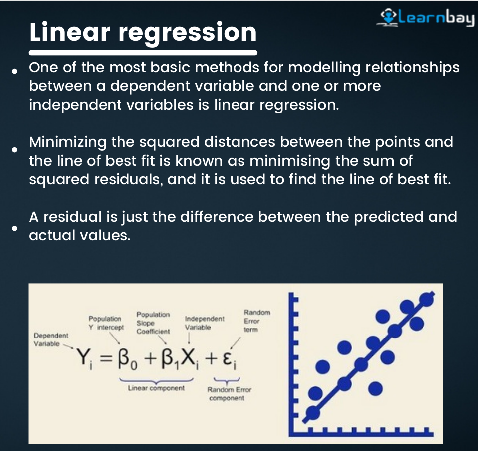 |
y = ax + b y = a0 + a1x1 + a2x2 + ⋯ LR is a good baseline regressor - can be fit very quickly and is very interpretable |
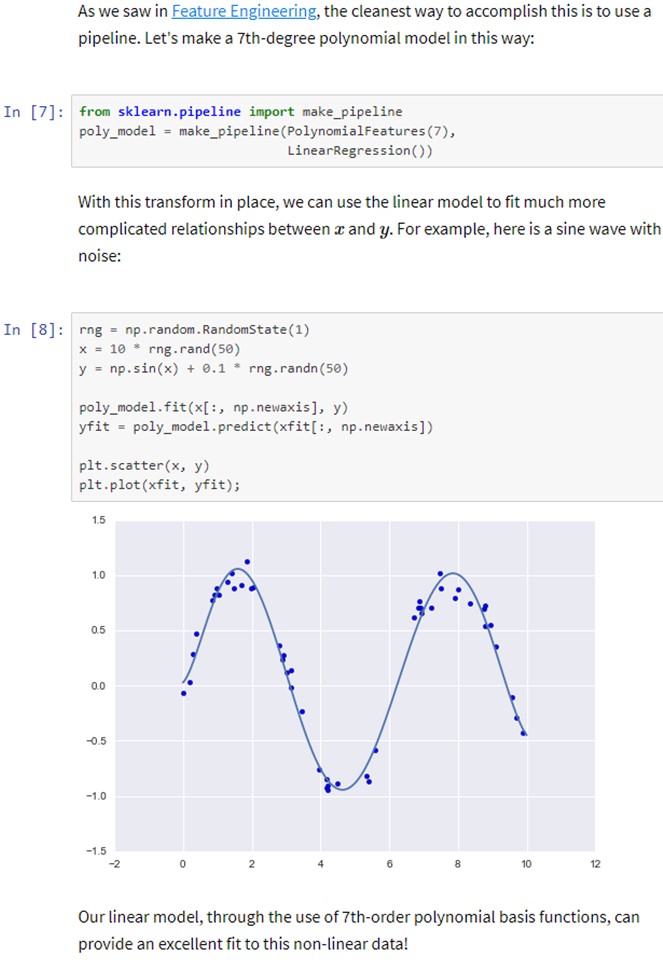
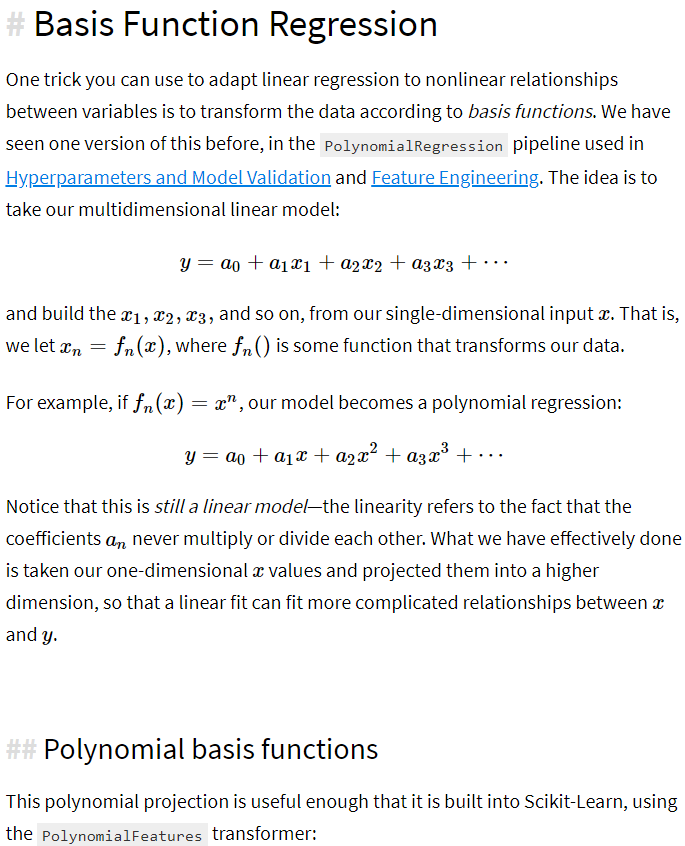
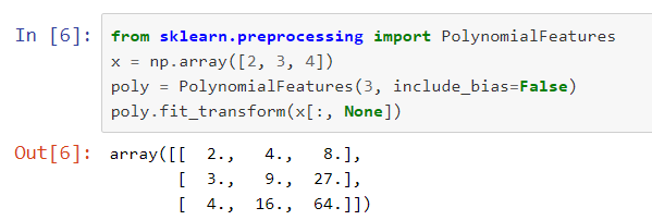
Polynomial and Other Basis Function Regressions
|
 |
How it works
A. Simpler explanation
https://towardsdatascience.com/machine-learning-basics-part-1-a36d38c7916
Goal - predict real-value variable y from a given pattern X, linear function:
ŷ = WX+b
X – vector of features, W - vector of weights (parameters) = extent of how each feature impacts the prediction, b - bias term.
Error of each example i :
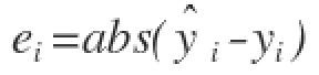
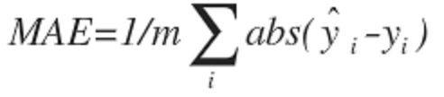
Cost functions (as an example) MAE or MSE:
 |
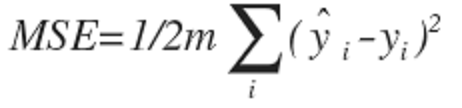 |
The MSE mean is halved (1/2) as a convenience to compute the gradient descent - the derivative of the square function will cancel out 1/2.
The main aim of training the ML algorithm is to adjust the weights W to reduce the error.
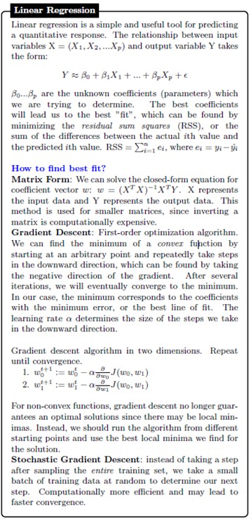
To minimize the error, the model while experiencing the examples of the training set, updates the model parameters W. These error calculations when plotted against the W is also called cost function J(w), since it determines the cost/penalty of the model. So minimizing the error is also called as minimization the cost function J.
Gradient descent Algorithm:
When we plot the cost function J(w) vs w. It is represented as below:
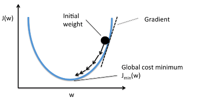
As we see from the curve, there exists a value of parameters W which has the minimum cost Jmin. Now we need to find a way to reach this minimum cost.
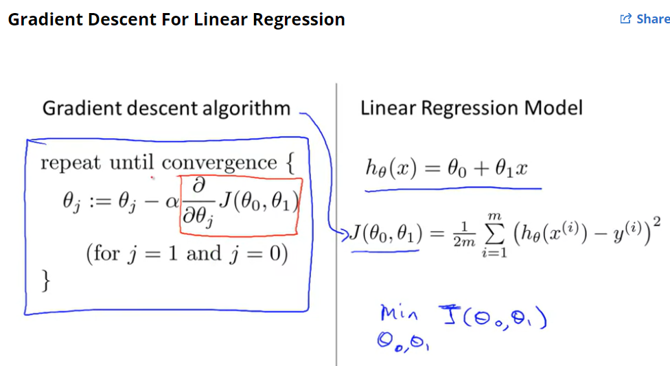
In gradient descent - start with random model parameters, calculate the error for each learning iteration, keep updating the model parameters to move closer to the values that results in minimum cost.

In the above equation we are updating the model parameters after each iteration. The second term of the equation calculates the slope or gradient of the curve at each iteration.
The gradient of the cost function is calculated as partial derivative of cost function J with respect to each model parameter wj, j takes value of number of features [1 to n]. α, alpha, is the learning rate, or how quickly we want to move towards the minimum. If α is too large, we can overshoot. If α is too small, means small steps of learning hence the overall time taken by the model to observe all examples will be more.
Types of doing gradient descent:
Batch gradient descent: use all training instances to update the model parameters in each iteration.
Mini-batch Gradient Descent: use only smaller size batches to update the model parameters in each iteration.
Stochastic Gradient Descent (SGD): use a random single training instance in each iteration. Often preferred to optimize cost functions when hundreds of thousands of training instances – converges quicker than batch gradient descent.
B. More complex (but similar) explanation
 |
 |
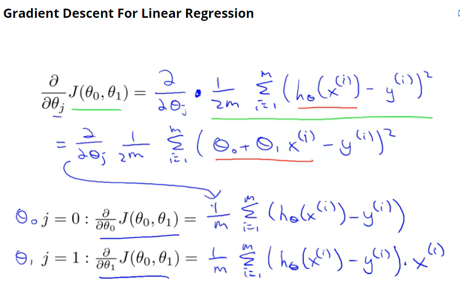
J in the equations above is the cost function. We are applying the gradient descent algorithm to minimize the cost function J (see Fig. 1 below), and for that we will define its derivative as shown on Fig. 2
Fig. 1 |
Fig. 2 |
Source: https://www.coursera.org/lecture/machine-learning/gradient-descent-for-linear-regression-kCvQc
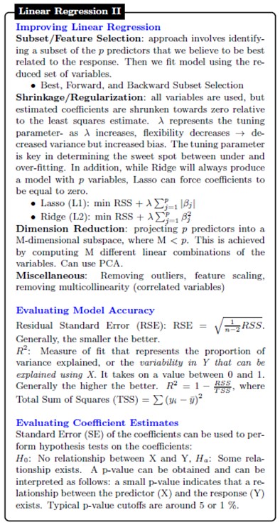
Ordinary Least Square Method (OLS)
Linear regression – modeling approach while OLS – method to find simple linear regression of a set of data.
In statistics, ordinary least squares (OLS) or linear least squares is a method for estimating the unknown parameters in a linear regression model. This method minimizes the sum of squared vertical distances between the observed responses in the dataset and the responses predicted by the linear approximation.
How it works:
Set a difference between dependent variable and its estimation:
Square the difference:
Take summation for all data.
Minimize squared difference by taking partial derivative for each parameter and equate it with zero
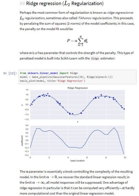
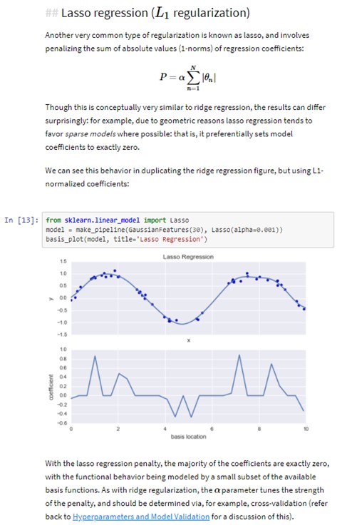
Avoid Overfitting - Regularization of LR
 |
 |
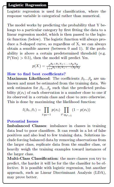
Logistic regression
 |
Additional theory
|
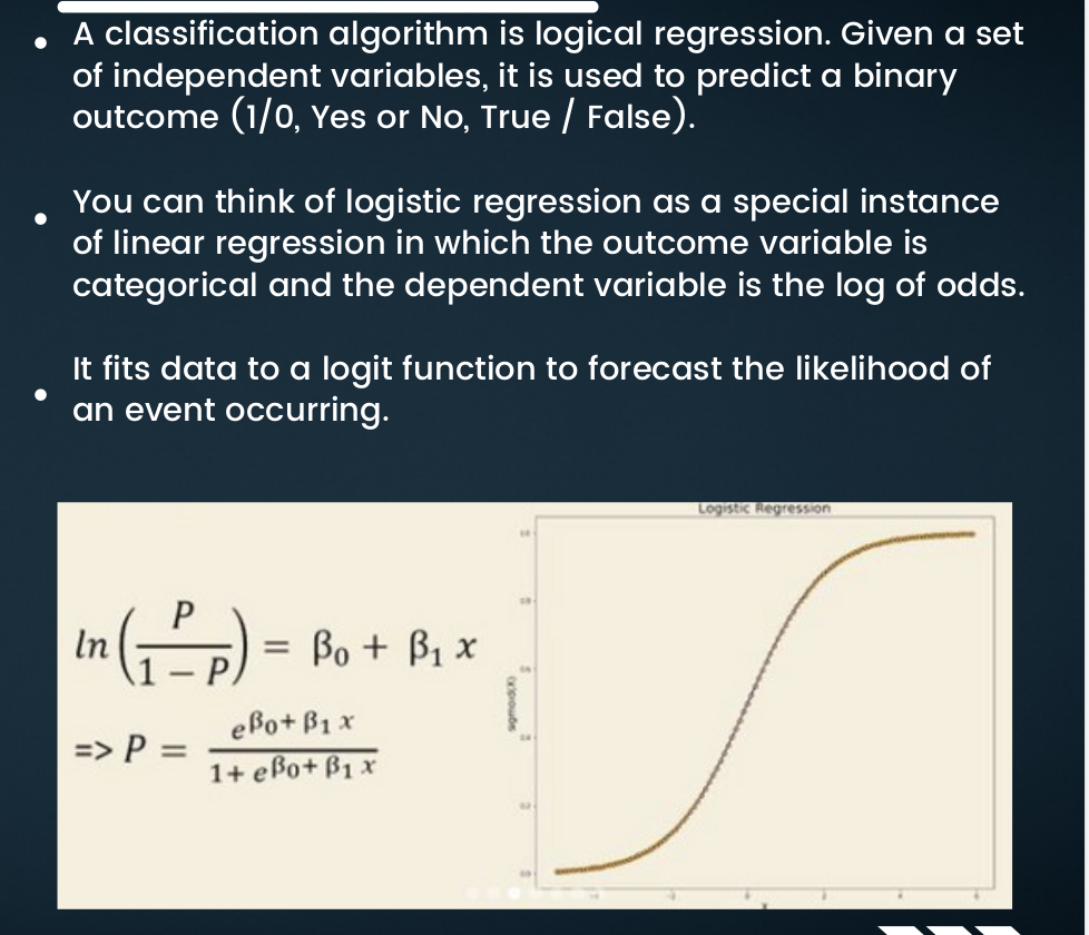
In logistic regression, the response variable describes the probability that the outcome is the positive case (if prob > discrimination threshold).
Cost Function – Cross-Entropy
We cannot use the same cost function that we used for linear regression because the Sigmoid Function will cause the output to be wavy, causing many local optima. In other words, it will not be a convex function.
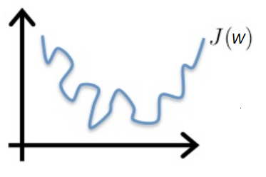 In order to ensure the cost function is convex (and therefore ensure convergence to the global minimum), the cost function is transformed using the logarithm of the sigmoid function. The cost function for logistic regression looks like:
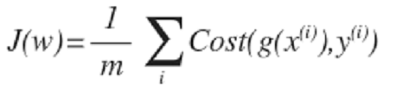


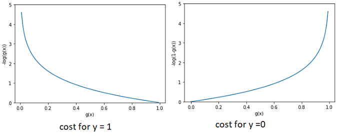
So the cost function for logistic regression is:
 Since the cost function is a convex function, we can run the gradient descent algorithm to find the minimum cost.