How do neural networks learn ?
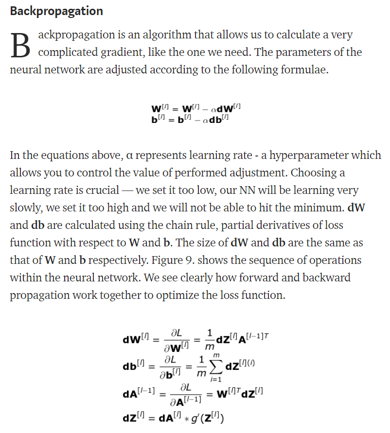
The learning process is about updating the values of weights matrix W and biases vector b to find a loss function minimum by using gradient descent through partial derivatives of loss function. Derivatives describe the slope of the function, and thus we know how to manipulate variables in order to move downhill. Alpha = learning rate (important to set it right). W & b are adjusted to get down the slope in the right direction. |
 |
Note:
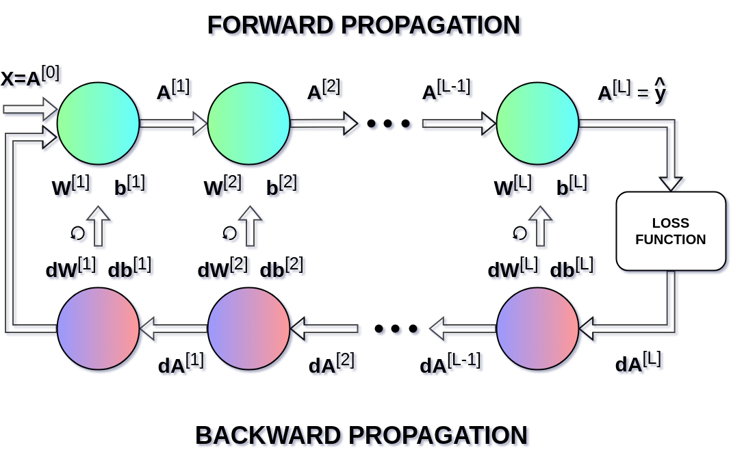
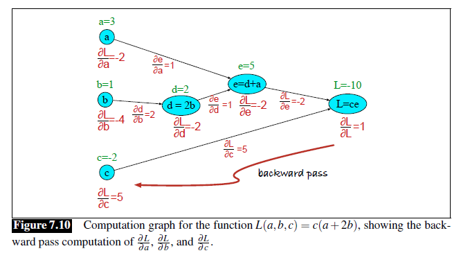
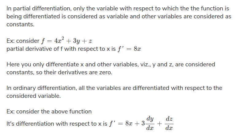 Backpropagation involves taking the loss function’s error rate (e.g. MSE) between true values and computed values of a forward propagation and iteratively feeding it backward through the neural network layers to adjusts the weights and biases until the error rate reaches a minimum so that a NN can use randomly allocated weights and biases to produce the correct output.
After each forward pass, the backward pass adjusts weights and biases to minimize the loss function C. This is done by computing the gradient of C with respect to each weight which tells you how much the parameter x needs to change to minimize C (see gradient) and whether to increase (negative gradient) or decrease (positive gradient) the weights.
The DL Training Process
Initialization and objective. Training begins with a labeled dataset and a network’s weights initialized randomly. Training is the iterative process of updating those weights via gradient-based optimization to minimize a loss function that quantifies prediction error.
Mini-batch training. Rather than processing the full dataset at once (batch gradient descent) or one example at a time (stochastic gradient descent), training typically uses mini-batch stochastic gradient descent: a subset of examples (a mini-batch, typically tens to thousands of samples) is processed per step — forward pass, loss computation, backpropagation, parameter update. One full pass through the dataset is an epoch; training runs for many epochs.
Forward pass. Input data propagates through the network layer by layer. Each layer applies an affine transformation (a weighted linear combination of inputs plus a bias term, parameterized by a weight matrix) followed by a nonlinear activation function (e.g., ReLU, GELU, sigmoid). The nonlinearity is essential: without it, stacked layers would collapse into a single linear transformation. Successive layers learn progressively more abstract representations (hierarchical feature learning), from low-level features toward task-relevant, high-level abstractions, culminating in the output layer's prediction.
Activation caching. During the forward pass, intermediate layer outputs (activations) are cached in memory, since they are required to compute gradients during backpropagation. This is the primary reason training consumes substantially more memory than inference — inference discards activations immediately (no backward pass).
Loss computation. The network's output is compared against ground-truth labels using a loss function (e.g., cross-entropy loss for classification, mean squared error for regression), producing a single scalar value representing aggregate error over the batch. Loss func depends on training objective.
Backpropagation. Gradients of the loss with respect to every weight are computed via backpropagation, an efficient application of the chain rule of calculus applied recursively from the output layer back to the input layer. Each weight's gradient — a vector quantity representing the partial derivative of the loss with respect to that weight — indicates the direction and magnitude of change that would most increase the loss (or, negated, most decrease it). This process is the solution to determine each parameter's contribution to the total error. Cached activations from the forward pass are consumed here, since a weight's gradient depends on the input that passed through it.
Backpropagation is cheap because it computes gradients for all parameters in a single backward sweep (there is one error signal and millions of weights), exploiting shared intermediate computations instead of re-computing them per weight, at roughly 2x the computational cost of the forward pass alone. This efficiency (linear, not exponential in the number of params) is what makes training large-scale networks computationally tractable.
Trainable vs. non-trainable elements. Only learnable parameters — weight matrices, biases, embedding tables, and normalization scale/shift parameters — are updated. Inputs are fixed data, not parameters. Activations are transient intermediate values, discarded after use. Layers that are deliberately frozen (parameters excluded from the update step) are skipped during the backward update — the mechanism underlying parameter-efficient fine-tuning (PEFT) methods such as LoRA, which train only a small number of additional parameters while keeping the base model frozen.
Parameter update (gradient descent). Picture the loss as a landscape of hills and valleys, where each location represents one possible setting of all the weights, and the altitude at that location is how wrong the model is. Low points are good — they're settings where the model performs well. Training is the process of walking downhill toward one of those low points. The catch: we can't see the whole landscape at once, only the ground right under our feet. The gradient tells us which direction is steepest uphill from where we're standing; we just step in the opposite direction — downhill. Take a small step, recompute the slope from the new spot, step again, and repeat. The learning rate governs the step size and is among the most critical hyperparameters: too large risks divergence or oscillation across the loss surface; too small risks impractically slow convergence.
Adaptive optimizers. Plain gradient descent has a problem: each mini-batch gives a slightly different, noisy reading of which way is downhill, since it only sees a small slice of the data. Stepping based on every noisy reading makes for a jittery, wandering walk. Momentum fixes this the way a rolling ball behaves on a bumpy slope: instead of reacting to each new slope reading in isolation, it keeps a running sense of the recent trend and keeps moving in that general direction, letting the noise from individual batches average out. The second idea is giving each weight its own step size. Some weights sit on steady, predictable terrain — same slope direction every time — so it's safe to take bigger steps there. Others sit on jumpy, erratic terrain, where big steps risk overshooting, so smaller steps are safer. Adaptive learning rate methods track how noisy each weight's history has been and scale its step size accordingly: confident strides where the ground is reliable, cautious steps where it isn't. Adam, the most widely used optimizer, combines both ideas — momentum for smoothing, plus per-weight adaptive step sizes. The cost is memory: Adam has to keep two running trackers for every single weight in the model (one for the momentum trend, one for the noise level), which is a big reason training a model takes far more memory than just running it
Learning rate scheduling. Training runs typically follow a learning rate schedule: a warmup phase of small learning rates while optimizer state estimates are still unreliable, followed by a period at peak learning rate, then a decay phase (linear, cosine, or step decay) as training progresses, allowing convergence to a stable minimum rather than oscillation around it. Data is typically shuffled each epoch to prevent the model from learning spurious patterns tied to example ordering.
Gradient clipping. To prevent instability from anomalously large gradients (which could cause a destructively large parameter update), gradient clipping caps the norm or magnitude of the gradient before the update is applied. This is standard practice, particularly for large-scale models.
Monitoring and diagnostics. Training is monitored via training loss and validation loss (error on held-out data). Both decreasing indicates effective learning. Training loss decreasing while validation loss increases indicates overfitting — the model is memorizing training data rather than generalizing — signaling a need for regularization or early stopping. Neither decreasing suggests a bug in the model, hyperparameters, or data pipeline; a standard diagnostic is the single-batch overfitting test — verifying the model can drive loss to near-zero on one small batch, since failure to do so indicates an implementation bug rather than a modeling issue.
Summary. The full training loop — forward pass, loss computation, backpropagation, parameter update — repeats for many iterations, incorporating warmup, adaptive optimization, learning rate decay, and gradient clipping, while validation metrics are monitored to ensure generalization. The broader landscape of deep learning techniques — architectures, optimizers, normalization, regularization — exists largely to make this core loop stable, efficient, and effective
Activation Functions
https://towardsdatascience.com/activation-functions-neural-networks-1cbd9f8d91d6
Without them, neural network = combination of linear functions = linear function itself => limited expansiveness similar to logistic regression. The non-linearity element allows for greater flexibility and creation of complex functions during the learning process. The choice of activation function can significantly influence the network's learning capabilities, efficiency, and suitability for specific tasks like binary or multi-class classification.
The sigmoid activation function is particularly useful for binary classification in the output layer due to its output range [0,1], aligning well with probability interpretation. However, its susceptibility to the vanishing gradient problem can hinder learning in deep networks, making it less favorable for hidden layers.
Tanh shares similarities with sigmoid but outputs values between [-1,1], offering a centered range that can lead to faster convergence in some cases. It is also prone to vanishing gradients, but to a lesser extent which makes it a somewhat better choice for hidden layers.
ReLU, with its simple thresholding at zero, is highly effective in hidden layers due to computational efficiency and mitigation of the vanishing gradient problem. However, the dying ReLU issue, where neurons permanently output zeros, can impede learning.
Leaky ReLU addresses the dying ReLU problem by allowing a small, positive gradient for negative inputs, promoting continuous learning and maintaining ReLU's advantages for positive inputs. This is a robust choice for hidden layers, but the additional hyperparameter α requires tuning.
Softmax is indispensable for multi-class classification tasks in the output layer, converting logits to probabilities summing to one. It's well-suited for scenarios with mutually exclusive classes, providing a clear probabilistic interpretation. However, its drawbacks include computational complexity and potential for numerical instability due to exponentiation.
In summary, the choice between ReLU, sigmoid, tanh, Leaky ReLU, and Softmax depends on the specific requirements of the task, including the network architecture and the nature of the ML problem, and is made based on experimentation and validation.
REVIEW THE GWU DL / NLP COURSE FOR MORE CORE BASIC INSIGHTS – VERY HELPFUL REFRESHER LECTURE NOTES!
Transfer Functions to determine the output of a node, map the resulting values to a range: ( [0, 1], [-1, 1], etc. depending on the function). Two types: linear and non-linear
Linear or Identity Activation Function
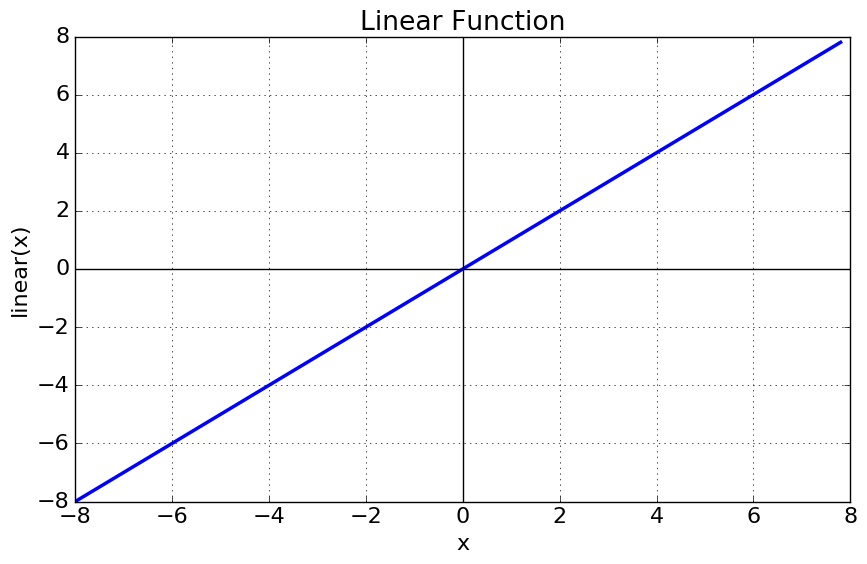
Fig: Linear Activation Function
f(x) = x, [ -inf, inf ]
Doesn’t help with complexity or various aspects of data fed to NN, but is used in output layers of regression models, autoencoders, special cases where no transformation is desired, simplified / baseline models -
making the model just a weighted sum of inputs.
Non-linear Activation Functions
Mostly used - nonlinearity helps the model to generalize / adapt to a variety of data and to differentiate between the output. Subtypes based on range and curves.
Main terms:
Derivative or Differential: Δy/Δx - change in y w.r.t. change in x (aka slope)
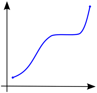
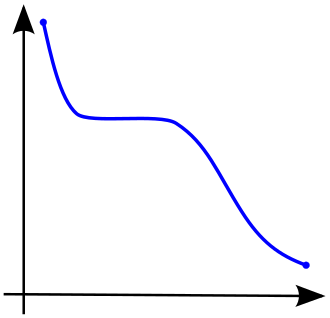
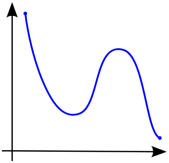
Monotonic f(x): either entirely non-increasing or non-decreasing.
f(x) = 2x + 3, f(x) = log(x), f(x) = e^x are increasing function;
f(x) = -x5, f(x) = e^-x are decreasing functions.
First derivative (which needs not be continuous) does not change sign.
 |
 |
 |
|---|---|---|
| Monotonically non-decreasing | Monotonically non-increasing | Non-monotonic |
Significance of monotonic functions in ML
In many applications, experts have prior knowledge about feature - target relationship (Credit Scoring: the higher the income, the risk of default should not increase. between income and the credit risk score ensures. Healthcare: a higher medication dose produces a stronger effect).
By incorporating monotonicity constraints (enforcing a monotonic relationship) the model predictions align with this intuition respecting these logical relationships, thereby increasing interpretability and trustworthiness.
Convex f(x): line segment between any two points of the function lies above or on the graph between the two points. y=x^2, y=e^x. In simple terms, a convex function is U-shaped, and a concave function is upside-down U-shaped. A twice-differentiable function of a single variable is convex if and only if its second derivative is nonnegative on its entire domain.
Convex f(x) – optimality in optimization problems
One of the most significant properties of convex functions is that any local minimum is also a global minimum => if you find a point where derivative (or gradient) = 0 – it’s the best possible solution globally. This greatly simplifies many optimization algorithms - eliminates the worry about getting “trapped” in sub-optimal local minima.
Convex problems have a well-behaved structure. Many optimization algorithms (e.g., gradient descent, Newton’s method, interior-point methods) are designed for or perform exceptionally well on convex problems.
In large-scale ML, where optimization is important, use of convex loss functions (squared error loss in regression or logistic loss in classification) leads to reliable and efficient algorithmic performance.
Concave f(x) - optimality in maximization problems
Concave functions have a similar benefit in maximization: any local maximum is a global maximum. Optimization methods (like gradient ascent or other maximization algorithms) will reliably identify the best possible solution without getting trapped in suboptimal local peaks.
Efficient Algorithms: many optimization algorithms can be tailored to either minimize a convex function or maximize a concave function. Numerous convex optimization methods are directly applicable to concave problems after an appropriate sign change.
Feed-forward ANN - wherein connections between nodes have no cycles / loops (different from RNNs). Was the first and simplest ANN where info moves forward: input nodes => hidden nodes => output nodes.
single-layer perceptron network - consists of a single layer of output nodes, the inputs are fed directly to the outputs via a series of weights (learns only linearly separable patterns, not capable of learning the concept of XOR),
multi-layer perceptron - multiple layers of computational units, usually interconnected in a feed-forward way,
CNNs.
1. Sigmoid / Logistic Act. F(x)
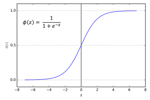
Fig: Sigmoid Function
S-shaped, range (0, 1)=> especially good for models predicting probability. Used in feed-forward nets. Differentiable - we can find slope of curve at any two points. Softmax extends it to multiclass tasks. Due to the first drawback below, it is still used in output layers, though largely replaced in hidden layers by ReLU/Tanh.
Drawbacks:
Monotonic, while its derivative is not (derivatives suffers from the vanishing gradient problem for large |x|, making deep networks harder to train). Can cause a neural network to get stuck during training.
Not zero-centered:
Outputs are always positive (0,1).
This can lead to inefficient gradient updates (zig-zagging in optimization)
2. Tanh / hyperbolic tangent Act. F(x)
f(z) = 
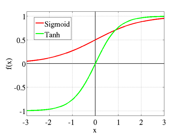
Tanh vs. Logistic Sigmoid
S-shaped, range (-1, 1). Unlike sigmoid, it is zero-centered: positive inputs mapped strongly positive, negative inputs mapped strongly negative, and the zero inputs mapped near zero.
Differentiable, monotonic while its derivative is not. Like sigmoid, saturates for large ∣x∣, causing very small [vanishing] gradients → training slows down in deep networks. Still useful in some RNNs (e.g., LSTMs/GRUs) and occasionally in hidden layers, but largely replaced by ReLU in deep feed-forward nets. Used mainly for binary classification in output layer of feed-forward nets.
3a. ReLU (Rectified Linear Unit) Act. F.
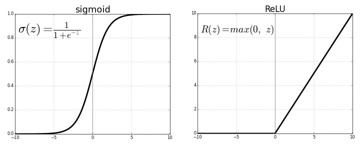
Fig: ReLU v/s Logistic Sigmoid
ReLU is half rectified (from bottom). f(x) = 0 if x < 0 and f(x) = x, if x >= 0
Range:[ 0, ∞]. Most used for CNNs or DL. Function and derivative are monotonic.
Advantages:
Computational efficiency: simple to compute (just thresholding at 0), which makes it fast and widely adopted.
Unlike sigmoid/tanh, ReLU does not saturate for positive inputs, which helps alleviate the vanishing gradient issue.
Disadvantages:
Disadvantage: negative values become zero immediately decreasing the ability to fit or train on data - negative values are not mapped appropriately on the plot.
“Dead ReLU” problem - neurons stop learning getting stuck in the negative region output 0 forever (gradient = 0).
Leaky ReLU, Parametric ReLU, ELU developed to fix the “dead ReLU” issue.
3b. Leaky ReLU
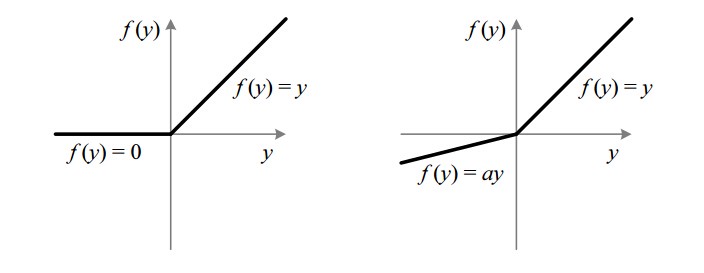
Fig : ReLU v/s Leaky ReLU
Attempt to solve the dying ReLU problem. Leak increases range. Usually, a= ~0.01. If it is not 0.01, f(x) is called randomized ReLU.
Range: [-inf, inf], both L. and R. ReLU & their derivatives are monotonic.
Advantage over ReLU:
Prevents neurons from dying (since gradient is never exactly 0 for x<0x < 0x<0).
Drawback:
Choosing the leak parameter a is arbitrary - too small still risks near-dead neurons, too large reduces nonlinearity.
3c. Softplus (SoftRELU)
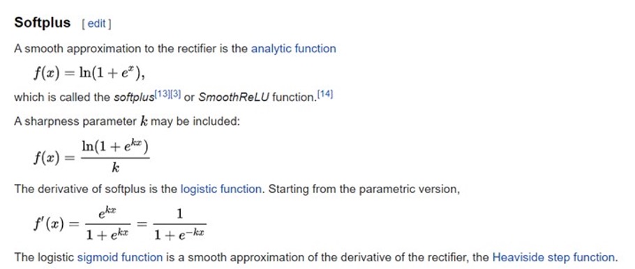
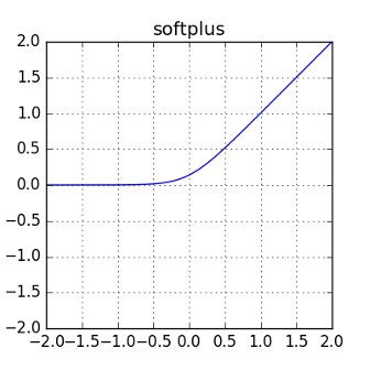
Range (0,∞).
Approximation to ReLU:
For large positive x, f(x)≈x. For large negative x, f(x)≈0.
Hence, it smoothly approximates ReLU avoiding the non-differentiability at 0.
Advantages over ReLU:
Differentiable everywhere (no “kink” at 0).
Avoids the “dead neuron” problem since negative inputs don’t map exactly to 0 (they map to small positive values).
Disadvantages:
Computationally more expensive than ReLU (involves logarithm + exponential).
Can suffer from vanishing gradients for very negative inputs (like sigmoid/tanh).
Use cases:
Not as widely used as ReLU, but appears in probabilistic models and networks where smoothness is desired (e.g., variational autoencoders).
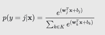
4. Softmax
Returns probability distribution for all classes: ratio of exponential of input parameter / sum of exponential parameters of all inputs. Multiclass unilabel classification. Multilabel uses multiple logistic regressions.
def softmax(scores):
return np.exp(scores)/sum(np.exp(scores)) # axis=0
 or
or 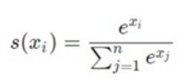
5. Maxout
An activation function that outputs the maximum value from a set of linear transformations. Given multiple affine transformations zi=xWi+bi, the output is: y=maxi(zi). Provides a piecewise linear approximation to arbitrary convex functions. Originally proposed for dropout networks; used in some GAN architectures. Benefits:
Improves model expressiveness.
Helps mitigate vanishing gradients.
Other activation f(x)
𝗣𝗥𝗲𝗟𝗨 (Parametric ReLU) - Similar to Leaky ReLU but the slope for negative values is learned during training rather than being predefined.
𝗘𝗟𝗨 (Exponential Linear Unit) - Tries to make the mean activations closer to zero. Negative inputs are transformed into values between -α and 0, slowing down the learning but producing a more robust model.
𝗦𝗘𝗟𝗨 (Scaled Exponential Linear Unit) - Like ELU, but with scaling, making it self-normalizing. It has specific conditions under which it can maintain mean 0 and variance 1.
GELU (Gaussian Error Linear Unit) - smoothly combines properties of ReLU and sigmoid by weighting inputs with their probability of being positive under a Gaussian distribution: GELU(x)=x⋅Φ(x) where Φ(x) is the standard normal CDF. It is widely used in Transformers (e.g., BERT, GPT) for better performance than ReLU or Tanh.
𝗦𝗼𝗳𝘁𝘀𝗶𝗴𝗻 - Divides the input by 1 plus the absolute value of the input. It's similar to tanh but is not widely used.
𝗛𝗮𝗿𝗱 𝗦𝗶𝗴𝗺𝗼𝗶𝗱 - A piecewise linear approximation of the sigmoid function, computationally more efficient than the regular sigmoid.
𝗦𝘄𝗶𝘀𝗵 (SiLU) - A self-gated activation function discovered by researchers at Google - combines linear & sigmoid behavior. Computationally efficient, found to work better than ReLU in some cases.
Hard swish – A piecewise linear approximation of Swish (faster, cheaper), often used in mobile/edge models. Keeps most of Swish’s accuracy benefits but at much lower compute cost.
𝗠𝗶𝘀𝗵 - A newer activation function that uses a combination of softplus and tanh functions. It has been shown to outperform many traditional activation functions in deep networks.
Why use derivatives (differentiation) in ML & DL?
When updating the curve, to know in which direction and how much to change / update the curve depending upon the slope.
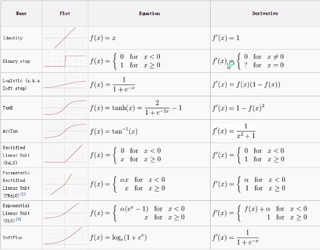
Fig: Activation Function Cheetsheet
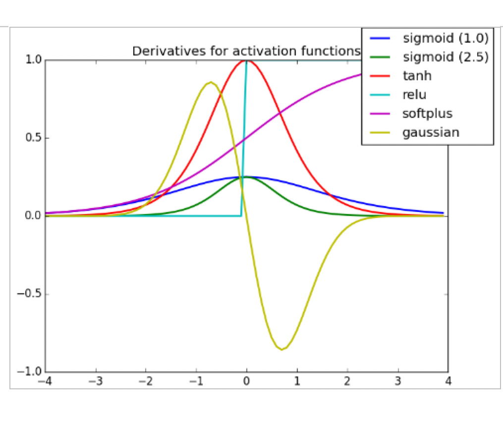 Fig: Derivative of Activation Functions
NORMALIZATION
Normalization keeps neural networks numerically stable, trainable at scale, and often better at generalizing. Core goals:
Stabilize training
Prevent exploding/vanishing activations.
Keep activations in a “healthy” range (not too big, not too small).
Improve gradient flow
Smoother loss landscape → makes backpropagation more effective.
Reduces internal covariate shift (shifts in activation distributions as training progresses).
Speed up convergence
Networks train faster with fewer epochs.
Optimizers (like SGD, Adam) behave more reliably.
Improve generalization
Acts as a form of regularization (e.g., BatchNorm adds noise through batch statistics).
Helps models avoid overfitting.
Enable very deep architectures
Without normalization, extremely deep models (ResNets, Transformers, GANs) would be nearly impossible to train effectively.
Batch Normalization (BN)
Definition: Normalizes activations across the batch dimension and features.
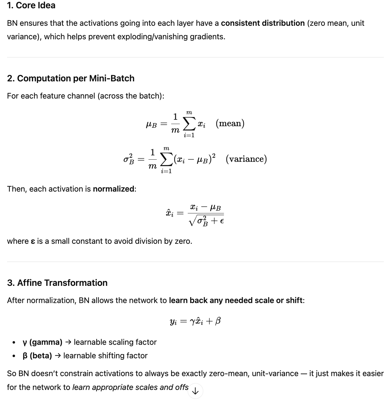
How it works: For each feature channel, it computes the mean and variance across the entire mini-batch, then rescales and shifts (subtracts mean and divide by standard deviation).
Strengths: Improves training stability, accelerates convergence.
Limitations: Depends on batch size; performance drops with very small batches.
Input shape: [B, C, H, W]
Normalize across: B, H, W (per channel C)
-------------------------------------------------
For each channel:
Mean/Var computed over all batch samples + spatial positions
Layer Normalization (LN)
Definition: Normalizes across all features of a single sample (not across the batch).
How it works: For each data point, compute mean and variance over all hidden units in a layer.
Strengths: Independent of batch size; commonly used in NLP (e.g., Transformers).
Limitations: May not perform as well as BN in CNNs.
Input shape: [B, C, H, W]
Normalize across: C, H, W (per sample B)
-------------------------------------------------
For each individual sample:
Mean/Var computed across all features in the layer
RMSNorm (Root Mean Square Layer Normalization) - simplified variant of Layer Normalization that normalizes using only the root mean square (RMS) of activations, without centering (no mean subtraction).
Instance Normalization (IN)
Definition: Normalizes each individual feature map per sample, across spatial dimensions.
How it works: For each channel in a single instance, compute mean and variance across spatial positions.
Strengths: Popular in image style transfer tasks, as it removes instance-specific contrast.
Limitations: Less effective for tasks requiring strong batch-level statistics.
Input shape: [B, C, H, W]
Normalize across: H, W (per channel C, per sample B)
-------------------------------------------------
For each channel of each sample:
Mean/Var computed over spatial positions only
In Instance Normalization (IN), the term “instance” refers to a single sample in the batch (e.g., one image), normalized independently from all the others.
Let’s unpack it:
Suppose your input to the network is shaped [B, C, H, W], where
B = batch size (number of instances)
C = number of channels (e.g., RGB = 3, or deep feature maps)
H, W = spatial dimensions
In Instance Normalization, normalization is applied individually per instance (per image), and per channel.
That means: for each image in the batch, and for each channel in that image, the mean and variance are computed only over the spatial dimensions (H, W).
It does not mix information across the batch (like BatchNorm) and does not mix channels together (like LayerNorm).
✅ Intuition in style transfer:
Each image (instance) may have very different contrast/lighting. Normalizing each instance separately removes this contrast variation, making it easier to apply a consistent “style” to the image, regardless of the original lighting.
Group Normalization (GN)
Definition: Divides feature channels into groups and normalizes within each group for each sample.
How it works: Computes mean and variance over a subset of channels grouped together.
Strengths: Works well with small batch sizes (unlike BN); balances between LN and IN.
Limitations: Requires choosing the number of groups as a hyperparameter.
Input shape: [B, C, H, W]
Normalize across: Subset of channels (C/G) + H, W (per group, per sample B)
-------------------------------------------------
Channels are divided into G groups:
Mean/Var computed within each group
PixelNorm (Pixelwise Normalization)
A normalization technique applied per pixel (spatial location), across all channels.
Purpose: Ensures each pixel has unit norm across channels.
Benefits:
Used in Progressive GANs to stabilize training.
Removes the need for batch statistics.
✅ Key Difference Summary:
BN → normalize across the whole batch (+ spatial dimensions) → good for large batches; fails w/small ones. Improves stability, accelerates training
LN → normalize across the all features of a single sample → good for NLP, Transformers (batch-independent - works with any batch siz). Less effective in CNNs
IN → normalize each channel separately, per sample (instance) → good for image style transfer. Removes instance-specific contrast. Weaker for recognition/classification.
GN → normalize across groups of channels per sample → more flexible, good for [vision models with] small batches, but requires tuning group size. Works well regardless of batch size, balances BN & LN.
Other normalization techniques
Spectral Normalization
Definition: A weight normalization technique that rescales the weight matrix of each layer by its largest singular value (spectral norm).
How it works:
For a weight matrix W, compute its largest singular value σ(W).
Normalize as WSN=W/σ(W).
Purpose:
Controls the Lipschitz constant of the network → stabilizes training.
Especially important in GANs, where it prevents discriminator from becoming too strong and destabilizing training.
Benefit: Stabilizes adversarial training, prevents exploding activations.
Weight Normalization
Definition: A reparameterization of weight vectors into a magnitude and direction component.
How it works:
For weight vector w, reparameterize as:
w=g / ∥v∥v
where g is a learnable scalar (magnitude) and v is a learnable vector (direction).
Purpose:
Decouples the length (scale) and direction of weights, making optimization easier.
Improves convergence speed in stochastic gradient descent.
Benefit: Often speeds up training and stabilizes optimization (but less commonly used now compared to BatchNorm or LayerNorm).
✅ Key Difference:
Spectral Normalization: Normalizes weights by their largest singular value → stabilizes Lipschitz continuity (common in GANs).
Weight Normalization: Reparameterizes weights into scale + direction → improves optimization dynamics (general training).
Example - How Batch Normalization works:
Process and add to this primer:
Neural networks simplified: https://towardsai-net.cdn.ampproject.org/c/s/towardsai.net/p/l/step-by-step-basic-understanding-of-neural-networks-with-keras-in-python?amp=1
Regularization: https://blog.datadive.net/selecting-good-features-part-ii-linear-models-and-regularization/