Loss Functions
https://machinelearningmastery.com/loss-and-loss-functions-for-training-deep-learning-neural-networks/
Shows how far we are from the ‘ideal’ solution - with each iteration the value of the loss function decreases and accuracy increases (red&blue plots).
ML algorithms optimize (minimize or maximize) an objective function, called otherwise a loss function / cost function (minimization), utility / fitness function (maximization), energy function[al]. Solution sought - optimal solution. Optimization allows to learn to reduce the error in prediction in conventional optimization problems – minimization.
Most common method to find a function’s minimum - gradient descent. In practice, it is often convenient to work with the natural logarithm of the likelihood function, called the log-likelihood. There is not a single loss function that works for all kind of data. It depends on a number of factors including the presence of outliers, choice of machine learning algorithm, time efficiency of gradient descent, ease of finding the derivatives and confidence of predictions
Under this framework, the choice of loss function depends on the activation function in the output layer. Both depend on the framing of the prediction problem. Most of the time, we use the cross-entropy between the data distribution and the model distribution, but the output representation determines the form of the cross-entropy function.
Regression functions predict a continuous value (quantity), and classification functions predict a label
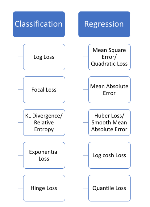
Selecting loss function
Binary Classification
Output Layer: One node with a sigmoid activation unit.
Loss Function: Cross-Entropy (Log loss)
Multi-Class Classification
Output Layer: One node for each class using the softmax activation function.
Loss Function: Cross-Entropy (Log loss)
Regression
Predict a real-value quantity.
Output Layer: One node with a linear activation unit
Loss Function: Mean Squared Error (MSE), MAE, MBE
Common Loss Functions
https://towardsdatascience.com/common-loss-functions-in-machine-learning-46af0ffc4d23
https://heartbeat.fritz.ai/5-regression-loss-functions-all-machine-learners-should-know-4fb140e9d4b0
A. Classification
Hinge Loss / Multi class SVM Loss

Score of correct category should be greater than sum of scores of all incorrect categories by some safety margin (usually one) => used for maximum-margin classification - support vector machines. Not differentiable, but is convex => makes it easy to work w/usual convex optimizers in ML.
Example:
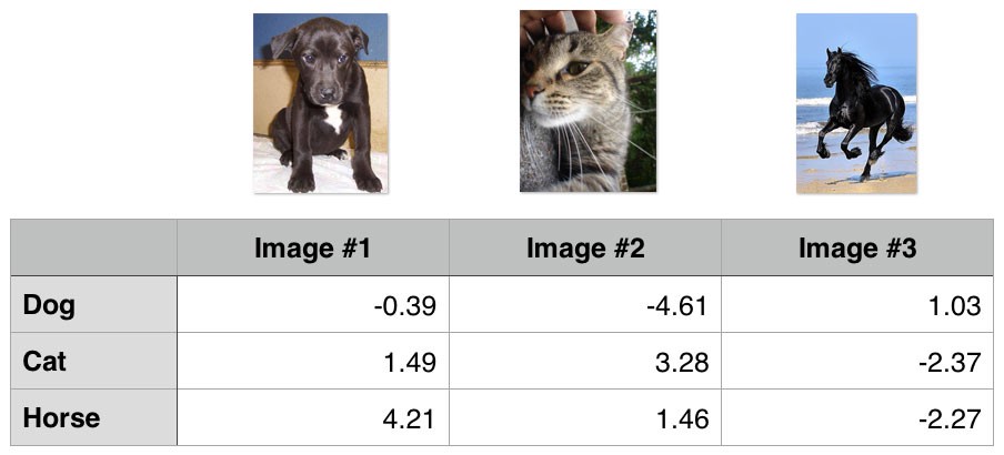
Hinge losses:
## 1st training example
max(0, (1.49) - (-0.39) + 1) + max(0, (4.21) - (-0.39) + 1)
max(0, 2.88) + max(0, 5.6)
2.88 + 5.6
8.48 (High loss as very wrong prediction)
## 2nd training example
max(0, (-4.61) - (3.28)+ 1) + max(0, (1.46) - (3.28)+ 1)
max(0, -6.89) + max(0, -0.82)
0 + 0
0 (Zero loss as correct prediction)
## 3rd training example
max(0, (1.03) - (-2.27)+ 1) + max(0, (-2.37) - (-2.27)+ 1)
max(0, 4.3) + max(0, 0.9)
4.3 + 0.9
5.2 (High loss as very wrong prediction)
Cross Entropy Loss/Negative Log Likelihood
The binary cross-entropy (BCE) loss is otherwise known as Logistic Loss (Log Loss)
1) Pointwise BCE loss (per sample):

2) Batch BCE Loss (average – uses sigmoid):

3) Categorical cross-entropy (more than 2 categories – uses softmax):
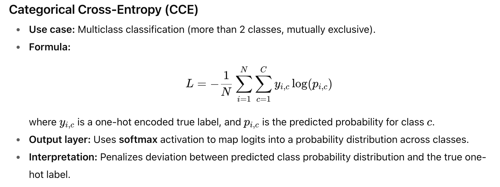
Estimated between a distribution of true and predicted values. Most common, increases as predicted probability diverges from actual
If y(i) = 1, second half of f(x) disappears, while if y(i) = 0, first half disappears. We are multiplying the log of the actual predicted probability for the ground truth class. Cross entropy loss penalizes predictions that are confident, but wrong.
import numpy as np
def cross_entropy(predictions, targets, epsilon=1e-10):
predictions = np.clip(predictions, epsilon, 1. - epsilon)
N = predictions.shape[0]
ce_loss = -np.sum(np.sum(targets * np.log(predictions + 1e-5)))/N
return ce_loss
predictions = np.array([[0.25,0.25,0.25,0.25], [0.01,0.01,0.01,0.96]])
targets = np.array([[0,0,0,1], [0,0,0,1]])
cross_entropy_loss = cross_entropy(predictions, targets)
print ("Cross entropy loss is: " + str(cross_entropy_loss))
B. Regression
1. Mean Square Error / Quadratic Loss / L2 Loss
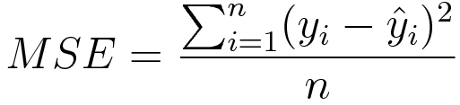
Average magnitude of error irrespective of their direction. Large prediction errors are penalized more due to squaring. It's easier to calculate gradients with MSE due to its mathematical properties.
import numpy as np
def rmse(predictions, targets):
differences = predictions - targets
differences_squared = differences ** 2
mean_of_differences_squared = differences_squared.mean()
rmse_val = np.sqrt(mean_of_differences_squared)
return rmse_val
y_hat = np.array([0.000, 0.166, 0.333])
y_true = np.array([0.000, 0.254, 0.998])
print("d is: " + str(["%.8f" % elem for elem in y_hat]))
print("p is: " + str(["%.8f" % elem for elem in y_true]))
rmse_val = rmse(y_hat, y_true)
print("rms error is: " + str(rmse_val))
2. Mean Absolute Error / L1 Loss
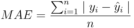
Measures magnitude of error without considering the direction. Unlike MSE, needs additional linear programming to compute gradients. More robust to outliers - doesn’t use square.
import numpy as np
def mae(predictions, targets):
differences = predictions - targets
absolute_differences = np.absolute(differences)
mean_absolute_differences = absolute_differences.mean()
return mean_absolute_differences
y_hat = np.array([0.000, 0.166, 0.333])
y_true = np.array([0.000, 0.254, 0.998])
print("d is: " + str(["%.8f" % elem for elem in y_hat]))
print("p is: " + str(["%.8f" % elem for elem in y_true]))
mae_val = mae(y_hat, y_true)
print ("mae error is: " + str(mae_val))
Mean Bias Error
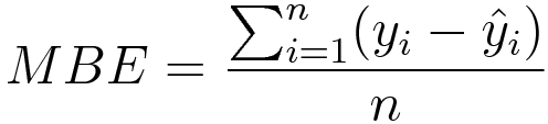
Less common. Less accurate - positive and negative errors can cancel each other out, but can help determine if model has positive or negative bias.
MSE vs. MAE (L2 loss vs L1 loss)
a) MSE - easier to solve
MSE - converges even with a fixed learning rate. Gradient of MSE loss decreases when the loss gets close to its minima - more precise at the end of training.
MAE - its derivatives are not continuous; its gradient is the same throughout => will be large even for small loss values => isn’t good for learning because it can miss minima at the end of training. Fix - dynamic learning rate which decreases when approaching the minima.
b) MAE - more robust / pays less attention to outliers, useful if the training data has a lot of them (huge negative/positive values in train set, but not in test set).
MSE loss gives more weight to outliers than a model with MAE loss because MSE squares the error.
Intuitively, if we need to make just one prediction, MSE tends to predict the mean of target values, while MAE - the median. And median is more robust to outliers.
c) Decide which one
If outliers are important business anomalies – use MSE. If they are noise / corrupted data – use MAE loss.
3. Huber Loss, Smooth MAE
Sometimes both MSE and MAE are not suitable for prediction: e.g. 90% of true target = 150, remaining 10% - between 0–30 => model w/MAE loss will predict 150 for all observations (median), but model w/MSE will be skewed towards the 0-30 range and make many predictions there. Both cases are undesirable.
Huber loss combines good properties from both MSE and MAE:
Less sensitive to outliers than MSE.
Differentiable at 0
It’s like absolute error, but becomes quadratic when error~0.
Huber loss approaches MSE when 𝛿~0 and MAE when 𝛿~∞ .

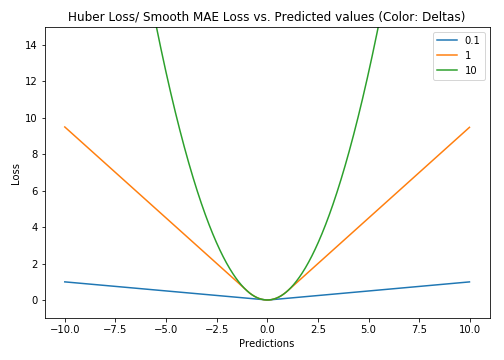
While MAE can miss minima at the end of training due to high gradient and MSE is more precise because its gradient decreases as the loss gets close to its minima, Huber loss curves around the minima which decreases the gradient + it’s more robust to outliers than MSE. If residuals > delta, behaves as L1 (less sensitive to outliers); if residuals < delta – behaves “appropriately” as L2.
Drawback - need to train hyperparameter delta. Choice of delta critical - determines what you’re willing to consider as an outlier.
4. Log-Cosh Loss
Logarithm of the hyperbolic cosine of the prediction error – also smoother than L2.
 Advantage: log(cosh(y_hat - y)) = approx. (x^2)/2 for small x and abs(x) – log(2) for large x => works mostly like MSE, but is not strongly affected by occasional wildly incorrect prediction. Has all advantages of Huber loss and, unlike Huber, is twice differentiable (ML models like XGBoost use Newton’s method to find the optimum – f(x) w/second derivative (Hessian) are more favorable).
Drawbacks: still suffers from the problem of gradient, Hessian for very large off-target predictions = constant => no splits for XGBoost.
5. Quantile Loss
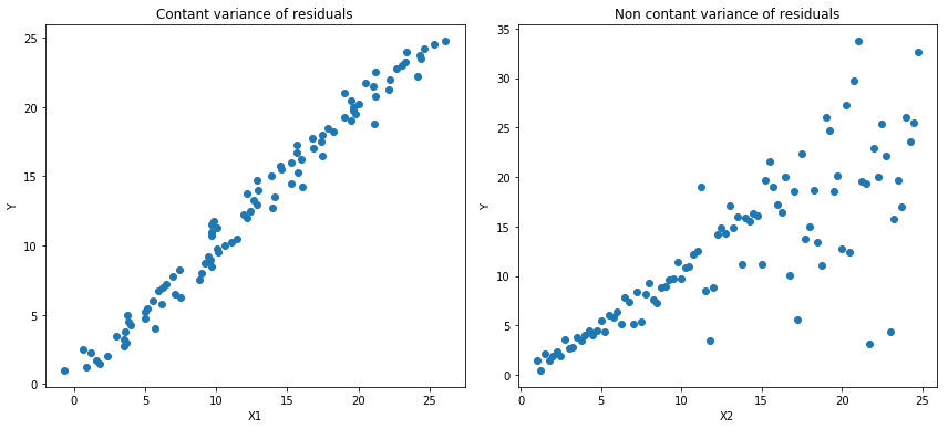
In most of the real-world prediction problems, we are often interested to know about the uncertainty in our predictions (improve decision making processes in business) – can be done by predicting the interval, not just point-wise predictions. But the least square regression, for example, is based on an assumption that residuals have constant variance across values of independent variables which is not always true in real life.
Regression based on quantile loss provides sensible prediction of intervals even for residuals (y — y_hat) with non-constant variance or non-normal distribution.
Quantile regression vs. Ordinary Least Square regression
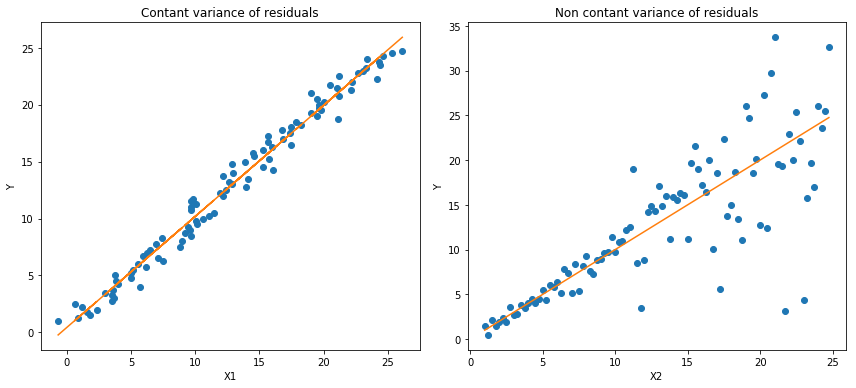
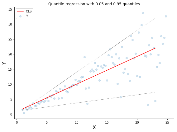
Quantile loss - extension of MAE (=MAE when the quantile is 50th percentile). Aims to estimate the conditional “quantile” of a response variable given certain values of predictor variables.
Idea – choose quantile value based on whether we give more value to positive errors or negative errors. Loss f(x) gives different penalties to overestimation and underestimation based on the chosen quantile (γ). E.g. quantile loss f(x) of γ = 0.25 penalizes overestimation and keeps predictions a little below median (γ in [0, 1]).
Used to calculate prediction intervals in NN and tree-based models.
.
___________________________________________________________________
References:
Sklearn example for gradient boosted tree regressors:
http://scikit-learn.org/stable/auto_examples/ensemble/plot_gradient_boosting_quantile.html - upper bound is constructed γ = 0.95 and lower bound using γ = 0.05Differences between L1 and L2 Loss Function and Regularization
Simulation study of loss functions. (Gradient boosting machines, a tutorial)
Regression prediction intervals using xgboost (Quantile loss)
Simulation study from [9]:
Demonstrates the properties of all above loss functions.
Simulated dataset sampled from asinc(x) function with Gaussian noise component ε ~N(0, σ2) and the impulsive noise component ξ ~ Bern(p) (the latter - to illustrate the robustness effect).
Observations from the simulations:
MAE is less affected by impulsive noise while MSE-based predictions are slightly biased.
Huber loss-based predictions are a little sensitive to the value of the hyperparameter delta.
Quantile loss - good estimation of corresponding confidence levels.
OTHER LOSS FUNCTIONS
Focal Loss → A modified cross-entropy loss that down-weights easy samples and focuses more on hard, misclassified examples (commonly used in object detection like RetinaNet).
Center Loss → Encourages features of the same class to cluster around a class center in embedding space, improving intra-class compactness.
Exponential Loss → The loss function used in AdaBoost; weights misclassified samples exponentially to focus on harder cases in subsequent rounds.
Contrastive Loss → Used in Siamese networks; minimizes distance between similar pairs and maximizes distance (above a margin) between dissimilar pairs.
Dice Loss → Based on the Dice coefficient; commonly used in segmentation tasks to maximize overlap between predicted and true masks.
Tversky Loss → A generalization of Dice loss for image segmentation that balances false positives and false negatives via tunable parameters.
InfoNCE Loss → A contrastive loss used in self-supervised learning; maximizes similarity between positive pairs while minimizing it against many negatives (used in SimCLR, CPC).
NT-Xent Loss (Normalized Temperature-Scaled Cross-Entropy) → A contrastive loss for self-supervised learning (SimCLR); uses softmax with temperature scaling to separate positive from negative pairs.
Pinball Loss → Used in quantile regression; penalizes overestimation and underestimation differently, depending on the target quantile.
Squared Hinge Loss → A variant of hinge loss (used in SVMs) that squares the margin violations, making the penalty smoother and more strongly penalizing misclassifications.
Triplet Loss → Ensures that an anchor sample is closer to a positive sample than to a negative sample by at least a margin, widely used in face recognition and metric learning.
Tukey Loss (Tukey’s Biweight Loss) → A robust regression loss that reduces the influence of outliers by flattening the penalty for very large residuals.
CV
ArcFace Loss → An angular margin–based softmax loss used in face recognition; enforces larger angular separation between classes for better discriminative features.
CosFace Loss → A cosine margin–based softmax loss for face recognition; imposes a margin in cosine space to enhance inter-class separability.
IoU Loss → Object detection loss that directly maximizes the Intersection-over-Union between predicted and ground-truth bounding boxes.
CIoU Loss (Complete IoU) → A bounding-box regression loss that combines IoU, center distance, and aspect ratio to improve localization accuracy in object detection.
DIoU Loss (Distance-IoU) → An object detection loss that adds a penalty based on the Euclidean distance between predicted and ground-truth box centers (faster convergence than IoU alone).
GIoU Loss (Generalized IoU) → An improvement over IoU loss for object detection; adds a penalty based on the area of the smallest enclosing box, helping when boxes don’t overlap.